EMD Trend [InvestorUnknown]EMD Trend is a dynamic trend-following indicator that utilizes Exponential Moving Deviation (EMD) to build adaptive channels around a selected moving average. Designed for traders who value responsive trend signals with built-in volatility sensitivity, this tool highlights directional bias, market regime shifts, and potential breakout opportunities.
How It Works
Instead of using standard deviation, EMD Trend employs the exponential moving average of the absolute deviation from a moving average—producing smoother, faster-reacting upper and lower bounds:
Bullish (Risk-ON Long): Price crosses above the upper EMD band
Bearish (Risk-ON Short): Price crosses below the lower EMD band
Neutral: Price stays within the channel, indicating potential mean reversion or low momentum
Trend direction is defined by price interaction with these bands, and visual cues (color-coded bars and fills) help quickly identify market conditions.
Features
7 Moving Average Types: SMA, EMA, HMA, DEMA, TEMA, RMA, FRAMA
Custom Price Source: Choose close, hl2, ohlc4, or others
EMD Multiplier: Controls the width of the deviation envelope
Bar Coloring: Candles change color based on current trend
Intra-bar Signal Option: Enables faster updates (with optional repainting)
Speculative Zones: Fills highlight aggressive momentum moves beyond EMD bounds
Backtest Mode
Switch to Backtest Mode for performance evaluation over historical data:
Equity Curve Plot: Compare EMD Trend strategy vs. Buy & Hold
Trade Metrics Table: View number of trades, win/loss stats, profits
Performance Metrics Table: Includes CAGR, Sharpe, max drawdown, and more
Custom Start Date: Select from which date the backtest should begin
Trade Sizing: Configure capital and trade percentage per entry
Signal Filters: Choose from Long Only, Short Only, or Both
Alerts
Built-in alerts let you automate entries, exits, and trend transitions:
LONG (EMD Trend) - Trend flips to Long
SHORT (EMD Trend) - Trend flips to Short
RISK-ON LONG - Price crosses above upper EMD band
RISK-OFF LONG - Price crosses back below upper EMD band
RISK-ON SHORT - Price crosses below lower EMD band
RISK-OFF SHORT - Price crosses back above lower EMD band
Use Cases
Trend Confirmation with volatility-sensitive boundaries
Momentum Entry Filtering via breakout zones
Mean Reversion Avoidance in sideways markets
Backtesting & Strategy Building with real-time metrics
Disclaimer
This indicator is intended for informational and educational purposes only. It does not constitute investment advice. Historical performance does not guarantee future results. Always backtest and use in simulation before live trading.
" TABLE "に関するスクリプトを検索

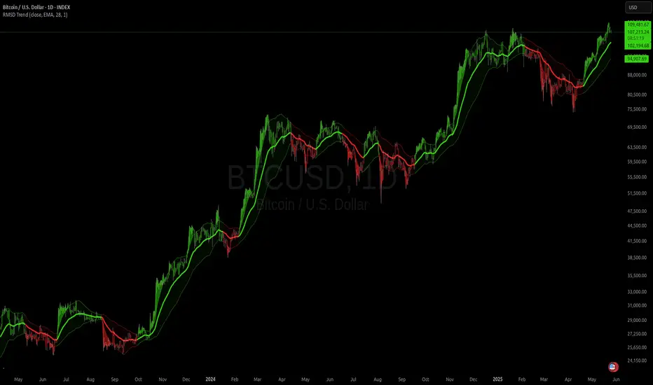
RMSD Trend [InvestorUnknown]RMSD Trend is a trend-following indicator that utilizes Root Mean Square Deviation (RMSD) to dynamically construct a volatility-weighted trend channel around a selected moving average. This indicator is designed to enhance signal clarity, minimize noise, and offer quantitative insights into market momentum, ideal for both discretionary and systematic traders.
How It Works
At its core, RMSD Trend calculates a deviation band around a selected moving average using the Root Mean Square Deviation (similar to standard deviation but with squared errors), capturing the magnitude of price dispersion over a user-defined period. The logic is simple:
When price crosses above the upper deviation band, the market is considered bullish (Risk-ON Long).
When price crosses below the lower deviation band, the market is considered bearish (Risk-ON Short).
If price stays within the band, the market is interpreted as neutral or ranging, offering low-risk decision zones.
The indicator also generates trend flips (Long/Short) based on crossovers and crossunders of the price and the RMSD bands, and colors candles accordingly for enhanced visual feedback.
Features
7 Moving Average Types: Choose between SMA, EMA, HMA, DEMA, TEMA, RMA, and FRAMA for flexibility.
Customizable Source Input: Use price types like close, hl2, ohlc4, etc.
Volatility-Aware Channel: Adjustable RMSD multiplier determines band width based on volatility.
Smart Coloring: Candles and bands adapt their colors to reflect trend direction (green for bullish, red for bearish).
Intra-bar Repainting Toggle: Option to allow more responsive but repaintable signals.
Speculation Fill Zones: When price exceeds the deviation channel, a semi-transparent fill highlights potential momentum surges.
Backtest Mode
Switching to Backtest Mode unlocks a robust suite of simulation features:
Built-in Equity Curve: Visualizes both strategy equity and Buy & Hold performance.
Trade Metrics Table: Displays the number of trades, win rates, gross profits/losses, and long/short breakdowns.
Performance Metrics Table: Includes key stats like CAGR, drawdown, Sharpe ratio, and more.
Custom Date Range: Set a custom start date for your backtest.
Trade Sizing: Simulate results using position sizing and initial capital settings.
Signal Filters: Choose between Long & Short, Long Only, or Short Only strategies.
Alerts
The RMSD Trend includes six built-in alert conditions:
LONG (RMSD Trend) - Trend flips from Short to Long
SHORT (RMSD Trend) - Trend flips from Long to Short
RISK-ON LONG (RMSD Trend) - Price crosses above upper RMSD band
RISK-OFF LONG (RMSD Trend) - Price falls back below upper RMSD band
RISK-ON SHORT (RMSD Trend) - Price crosses below lower RMSD band
RISK-OFF SHORT (RMSD Trend) - Price rises back above lower RMSD band
Use Cases
Trend Confirmation: Confirms directional bias with RMSD-weighted confidence zones.
Breakout Detection: Highlights moments when price breaks free from historical volatility norms.
Mean Reversion Filtering: Avoids false signals by incorporating RMSD’s volatility sensitivity.
Strategy Development: Backtest your signals or integrate with a broader system for alpha generation.
Settings Summary
Display Mode: Overlay (default) or Backtest Mode
Average Type: Choose from SMA, EMA, HMA, DEMA, etc.
Average Length: Lookback window for moving average
RMSD Multiplier: Band width control based on RMS deviation
Source: Input price source (close, hl2, ohlc4, etc.)
Intra-bar Updating: Real-time updates (may repaint)
Color Bars: Toggle bar coloring by trend direction
Disclaimer
This indicator is provided for educational and informational purposes only. It is not financial advice. Past performance, including backtest results, is not indicative of future results. Use with caution and always test thoroughly before live deployment.
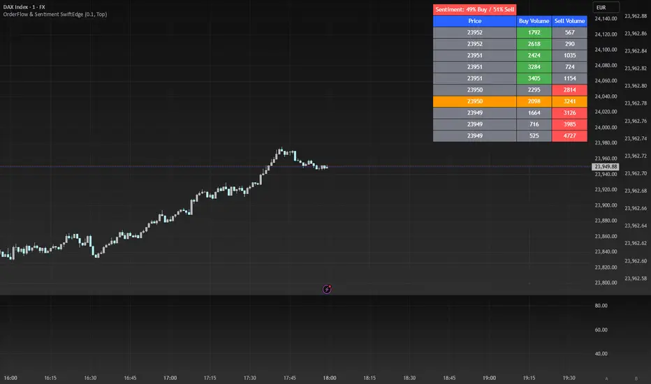
OrderFlow Sentiment SwiftEdgeOrderFlow Sentiment SwiftEdge
Overview
OrderFlow Sentiment SwiftEdge is a visual indicator designed to help traders analyze market dynamics through a simulated orderbook and market sentiment display. It breaks down the current candlestick into 10 price bins, estimating buy and sell volumes, and presents this data in an orderbook table alongside a sentiment row showing the buy vs. sell bias. This tool provides a quick and intuitive way to assess orderflow activity and market sentiment directly on your chart.
How It Works
The indicator consists of two main components: an Orderbook Table and a Market Sentiment Row.
Orderbook Table:
Simulates buy and sell volumes for the current candlestick by distributing total volume into 10 price bins based on price movement and proximity to open/close levels.
Displays the price bins in a table with columns for Price, Buy Volume, and Sell Volume, sorted from highest to lowest price.
Highlights the current price level in orange for easy identification, while buy and sell dominance is indicated with green (buy) or red (sell) backgrounds.
Market Sentiment Row:
Calculates the overall buy and sell sentiment (as a percentage) for the current candlestick based on the simulated orderflow data.
Displays the sentiment above the orderbook table, with the background colored green if buyers dominate or red if sellers dominate.
Features
Customizable Colors: Choose colors for buy (default: green), sell (default: red), and current price (default: orange) levels.
Lot Scaling Factor: Adjust the volume scaling factor (default: 0.1 lots per volume unit) to simulate realistic lot sizes.
Table Position: Select the table position on the chart (Top, Middle, or Bottom; default: Middle).
Default Properties
Positive Color: Green
Negative Color: Red
Current Price Color: Orange
Lot Scaling Factor: 0.1
Table Position: Middle
Usage
This indicator is ideal for traders who want to visualize orderflow dynamics and market sentiment in real-time. The orderbook table provides a snapshot of buy and sell activity at different price levels within the current candlestick, helping you identify areas of high buying or selling pressure. The sentiment row offers a quick overview of market bias, allowing you to gauge whether buyers or sellers are currently dominating. Use this information to complement your trading decisions, such as identifying potential breakout levels or confirming trend direction.
Limitations
This indicator simulates orderflow data based on candlestick price movement and volume, as TradingView does not provide tick-by-tick data. The volume distribution is an approximation and should be used as a visual aid rather than a definitive measure of market activity.
The indicator operates on the chart's current timeframe and does not incorporate higher timeframe data.
The simulated volumes are scaled using a user-defined lot scaling factor, which may not reflect actual market lot sizes.
Disclaimer
This indicator is for informational purposes only and does not guarantee trading results. Always conduct your own analysis and manage risk appropriately. The simulated orderflow data is an estimation and may not reflect real market conditions.
ETF Builder & Backtest System [TradeDots]Create, analyze, and monitor your own custom “ETF-like” portfolio directly on TradingView. This script merges up to 10 different assets with user-defined weightings into a single composite chart, allowing you to see how your personalized portfolio would have performed historically. It is an original tool designed to help traders and investors quickly gauge risk and return profiles without leaving the TradingView platform.
📝 HOW IT WORKS
1. Custom Portfolio Construction
Multiple Assets : Combine up to 10 different stocks, ETFs, cryptocurrencies, or other symbols.
User-Defined Weights : Allocate each asset a percentage weight (e.g., 15% in AAPL, 10% in MSFT, etc.).
Single Composite Value : The script calculates a weighted “ETF-style” price, effectively simulating a merged portfolio curve on your chart.
2. Performance Tracking & Return Analysis
Automatic History Capture : The indicator records each asset’s starting price when it first appears in your chosen date range.
Rolling Updates : As time progresses, all asset prices are continually evaluated and the portfolio value is updated in real time.
Buy & Hold Returns : See how each asset—and the overall portfolio—performed from the “start” date to the most recent bar.
Annualized Return : Automatically calculates CAGR (Compound Annual Growth Rate) to help visualize performance over varying timescales.
3. Table & Visual Output
Performance Table : A comprehensive table displays individual asset returns, annualized returns, and portfolio totals.
Normalized Chart Plot : The composite ETF value is scaled to 100 at the start date, making it easy to compare relative growth or decline.
Optional Time Filter : You can define a specific date range (Start/End Dates) to focus on a particular period or to limit historical data.
⚙️ KEY FEATURES
1. Flexible Asset Selection
Choose any symbols from multiple asset classes. The script will only run calculations when data is available—no need to worry about missing quotes.
2. Dynamic Table Reporting
Start Price for each asset
Percentage Weight in the portfolio
Total Return (%) and Annualized Return (%)
3. Simple Backtesting Logic
This script takes a straightforward Buy & Hold perspective. Once the start date is reached, the portfolio remains static until the end date, so you can quickly assess hypothetical growth.
4. Plot Customization
Toggle the main “ETF” plot on/off.
Alter the visual style for tables and text.
Adjust the time filter to limit or extend your performance measurement window.
🚀 HOW TO USE IT
1. Add the Script
Search for “ETF Builder & Backtest System ” in the Indicators & Strategies tab or manually add it to your chart after saving it in your Pine Editor.
2. Configure Inputs
Enable Time Filter : Choose whether to restrict the analysis to a particular date range.
Start & End Date : Define the period you want to measure performance over (e.g., from 2019-12-31 to 2025-01-01).
Assets & Weights : Enter each symbol and specify a percentage weight (up to 10 assets).
Display Options : Pick where you want the Table to appear and choose background/text colors.
3. Interpret the Table & Plots
Asset Rows : Each asset’s ticker, weighting, start price, and performance metrics.
ETF Total Row : Summarizes total weighting, composite starting value, and overall returns.
Normalized Plot : Tracks growth/decline of the combined portfolio, starting at 100 on the chart.
4. Refine Your Strategy
Compare how different weights or a new mix of assets would have performed over the same period.
Assess if certain assets contribute disproportionately to your returns or volatility.
Use the results to guide allocations in your real trading or paper trading accounts.
❗️LIMITATIONS
1. Buy & Hold Only
This script does not handle rebalancing or partial divestments. Once the portfolio starts, weights remain fixed throughout the chosen timeframe.
2. No Reinvestment Tracking
Dividends or other distributions are not factored into performance.
3. Data Availability
If historical data for a particular asset is unavailable on TradingView, related results may display as “N/A.”
4. Market Regimes & Volatility
Past performance does not guarantee similar future behavior. Markets can change rapidly, which may render historical backtests less predictive over time.
⚠️ RISK DISCLAIMER
Trading and investing carry significant risk and can result in financial loss. The “ETF Builder & Backtest System ” is provided for informational and educational purposes only. It does not constitute financial advice.
Always conduct your own research.
Use proper risk management and position sizing.
Past performance does not guarantee future results.
This script is an original creation by TradeDots, published under the Mozilla Public License 2.0.
Use this indicator as part of a broader trading or investment approach—consider fundamental and technical factors, overall market context, and personal risk tolerance. No trading tool can assure profits; exercise caution and responsibility in all financial decisions.

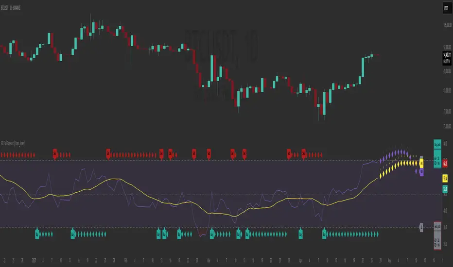
RSI Full Forecast [Titans_Invest]RSI Full Forecast
Get ready to experience the ultimate evolution of RSI-based indicators – the RSI Full Forecast, a boosted and even smarter version of the already powerful: RSI Forecast
Now featuring over 40 additional entry conditions (forecasts), this indicator redefines the way you view the market.
AI-Powered RSI Forecasting:
Using advanced linear regression with the least squares method – a solid foundation for machine learning - the RSI Full Forecast enables you to predict future RSI behavior with impressive accuracy.
But that’s not all: this new version also lets you monitor future crossovers between the RSI and the MA RSI, delivering early and strategic signals that go far beyond traditional analysis.
You’ll be able to monitor future crossovers up to 20 bars ahead, giving you an even broader and more precise view of market movements.
See the Future, Now:
• Track upcoming RSI & RSI MA crossovers in advance.
• Identify potential reversal zones before price reacts.
• Uncover statistical behavior patterns that would normally go unnoticed.
40+ Intelligent Conditions:
The new layer of conditions is designed to detect multiple high-probability scenarios based on historical patterns and predictive modeling. Each additional forecast is a window into the price's future, powered by robust mathematics and advanced algorithmic logic.
Full Customization:
All parameters can be tailored to fit your strategy – from smoothing periods to prediction sensitivity. You have complete control to turn raw data into smart decisions.
Innovative, Accurate, Unique:
This isn’t just an upgrade. It’s a quantum leap in technical analysis.
RSI Full Forecast is the first of its kind: an indicator that blends statistical analysis, machine learning, and visual design to create a true real-time predictive system.
⯁ SCIENTIFIC BASIS LINEAR REGRESSION
Linear Regression is a fundamental method of statistics and machine learning, used to model the relationship between a dependent variable y and one or more independent variables 𝑥.
The general formula for a simple linear regression is given by:
y = β₀ + β₁x + ε
β₁ = Σ((xᵢ - x̄)(yᵢ - ȳ)) / Σ((xᵢ - x̄)²)
β₀ = ȳ - β₁x̄
Where:
y = is the predicted variable (e.g. future value of RSI)
x = is the explanatory variable (e.g. time or bar index)
β0 = is the intercept (value of 𝑦 when 𝑥 = 0)
𝛽1 = is the slope of the line (rate of change)
ε = is the random error term
The goal is to estimate the coefficients 𝛽0 and 𝛽1 so as to minimize the sum of the squared errors — the so-called Random Error Method Least Squares.
⯁ LEAST SQUARES ESTIMATION
To minimize the error between predicted and observed values, we use the following formulas:
β₁ = /
β₀ = ȳ - β₁x̄
Where:
∑ = sum
x̄ = mean of x
ȳ = mean of y
x_i, y_i = individual values of the variables.
Where:
x_i and y_i are the means of the independent and dependent variables, respectively.
i ranges from 1 to n, the number of observations.
These equations guarantee the best linear unbiased estimator, according to the Gauss-Markov theorem, assuming homoscedasticity and linearity.
⯁ LINEAR REGRESSION IN MACHINE LEARNING
Linear regression is one of the cornerstones of supervised learning. Its simplicity and ability to generate accurate quantitative predictions make it essential in AI systems, predictive algorithms, time series analysis, and automated trading strategies.
By applying this model to the RSI, you are literally putting artificial intelligence at the heart of a classic indicator, bringing a new dimension to technical analysis.
⯁ VISUAL INTERPRETATION
Imagine an RSI time series like this:
Time →
RSI →
The regression line will smooth these values and extend them n periods into the future, creating a predicted trajectory based on the historical moment. This line becomes the predicted RSI, which can be crossed with the actual RSI to generate more intelligent signals.
⯁ SUMMARY OF SCIENTIFIC CONCEPTS USED
Linear Regression Models the relationship between variables using a straight line.
Least Squares Minimizes the sum of squared errors between prediction and reality.
Time Series Forecasting Estimates future values based on historical data.
Supervised Learning Trains models to predict outputs from known inputs.
Statistical Smoothing Reduces noise and reveals underlying trends.
⯁ WHY THIS INDICATOR IS REVOLUTIONARY
Scientifically-based: Based on statistical theory and mathematical inference.
Unprecedented: First public RSI with least squares predictive modeling.
Intelligent: Built with machine learning logic.
Practical: Generates forward-thinking signals.
Customizable: Flexible for any trading strategy.
⯁ CONCLUSION
By combining RSI with linear regression, this indicator allows a trader to predict market momentum, not just follow it.
RSI Full Forecast is not just an indicator — it is a scientific breakthrough in technical analysis technology.
⯁ Example of simple linear regression, which has one independent variable:
⯁ In linear regression, observations ( red ) are considered to be the result of random deviations ( green ) from an underlying relationship ( blue ) between a dependent variable ( y ) and an independent variable ( x ).
⯁ Visualizing heteroscedasticity in a scatterplot against 100 random fitted values using Matlab:
⯁ The data sets in the Anscombe's quartet are designed to have approximately the same linear regression line (as well as nearly identical means, standard deviations, and correlations) but are graphically very different. This illustrates the pitfalls of relying solely on a fitted model to understand the relationship between variables.
⯁ The result of fitting a set of data points with a quadratic function:
_________________________________________________
🔮 Linear Regression: PineScript Technical Parameters 🔮
_________________________________________________
Forecast Types:
• Flat: Assumes prices will remain the same.
• Linreg: Makes a 'Linear Regression' forecast for n periods.
Technical Information:
ta.linreg (built-in function)
Linear regression curve. A line that best fits the specified prices over a user-defined time period. It is calculated using the least squares method. The result of this function is calculated using the formula: linreg = intercept + slope * (length - 1 - offset), where intercept and slope are the values calculated using the least squares method on the source series.
Syntax:
• Function: ta.linreg()
Parameters:
• source: Source price series.
• length: Number of bars (period).
• offset: Offset.
• return: Linear regression curve.
This function has been cleverly applied to the RSI, making it capable of projecting future values based on past statistical trends.
______________________________________________________
______________________________________________________
⯁ WHAT IS THE RSI❓
The Relative Strength Index (RSI) is a technical analysis indicator developed by J. Welles Wilder. It measures the magnitude of recent price movements to evaluate overbought or oversold conditions in a market. The RSI is an oscillator that ranges from 0 to 100 and is commonly used to identify potential reversal points, as well as the strength of a trend.
⯁ HOW TO USE THE RSI❓
The RSI is calculated based on average gains and losses over a specified period (usually 14 periods). It is plotted on a scale from 0 to 100 and includes three main zones:
• Overbought: When the RSI is above 70, indicating that the asset may be overbought.
• Oversold: When the RSI is below 30, indicating that the asset may be oversold.
• Neutral Zone: Between 30 and 70, where there is no clear signal of overbought or oversold conditions.
______________________________________________________
______________________________________________________
⯁ ENTRY CONDITIONS
The conditions below are fully flexible and allow for complete customization of the signal.
______________________________________________________
______________________________________________________
🔹 CONDITIONS TO BUY 📈
______________________________________________________
• Signal Validity: The signal will remain valid for X bars .
• Signal Sequence: Configurable as AND or OR .
📈 RSI Conditions:
🔹 RSI > Upper
🔹 RSI < Upper
🔹 RSI > Lower
🔹 RSI < Lower
🔹 RSI > Middle
🔹 RSI < Middle
🔹 RSI > MA
🔹 RSI < MA
📈 MA Conditions:
🔹 MA > Upper
🔹 MA < Upper
🔹 MA > Lower
🔹 MA < Lower
📈 Crossovers:
🔹 RSI (Crossover) Upper
🔹 RSI (Crossunder) Upper
🔹 RSI (Crossover) Lower
🔹 RSI (Crossunder) Lower
🔹 RSI (Crossover) Middle
🔹 RSI (Crossunder) Middle
🔹 RSI (Crossover) MA
🔹 RSI (Crossunder) MA
🔹 MA (Crossover) Upper
🔹 MA (Crossunder) Upper
🔹 MA (Crossover) Lower
🔹 MA (Crossunder) Lower
📈 RSI Divergences:
🔹 RSI Divergence Bull
🔹 RSI Divergence Bear
📈 RSI Forecast:
🔹 RSI (Crossover) MA Forecast
🔹 RSI (Crossunder) MA Forecast
🔹 RSI Forecast 1 > MA Forecast 1
🔹 RSI Forecast 1 < MA Forecast 1
🔹 RSI Forecast 2 > MA Forecast 2
🔹 RSI Forecast 2 < MA Forecast 2
🔹 RSI Forecast 3 > MA Forecast 3
🔹 RSI Forecast 3 < MA Forecast 3
🔹 RSI Forecast 4 > MA Forecast 4
🔹 RSI Forecast 4 < MA Forecast 4
🔹 RSI Forecast 5 > MA Forecast 5
🔹 RSI Forecast 5 < MA Forecast 5
🔹 RSI Forecast 6 > MA Forecast 6
🔹 RSI Forecast 6 < MA Forecast 6
🔹 RSI Forecast 7 > MA Forecast 7
🔹 RSI Forecast 7 < MA Forecast 7
🔹 RSI Forecast 8 > MA Forecast 8
🔹 RSI Forecast 8 < MA Forecast 8
🔹 RSI Forecast 9 > MA Forecast 9
🔹 RSI Forecast 9 < MA Forecast 9
🔹 RSI Forecast 10 > MA Forecast 10
🔹 RSI Forecast 10 < MA Forecast 10
🔹 RSI Forecast 11 > MA Forecast 11
🔹 RSI Forecast 11 < MA Forecast 11
🔹 RSI Forecast 12 > MA Forecast 12
🔹 RSI Forecast 12 < MA Forecast 12
🔹 RSI Forecast 13 > MA Forecast 13
🔹 RSI Forecast 13 < MA Forecast 13
🔹 RSI Forecast 14 > MA Forecast 14
🔹 RSI Forecast 14 < MA Forecast 14
🔹 RSI Forecast 15 > MA Forecast 15
🔹 RSI Forecast 15 < MA Forecast 15
🔹 RSI Forecast 16 > MA Forecast 16
🔹 RSI Forecast 16 < MA Forecast 16
🔹 RSI Forecast 17 > MA Forecast 17
🔹 RSI Forecast 17 < MA Forecast 17
🔹 RSI Forecast 18 > MA Forecast 18
🔹 RSI Forecast 18 < MA Forecast 18
🔹 RSI Forecast 19 > MA Forecast 19
🔹 RSI Forecast 19 < MA Forecast 19
🔹 RSI Forecast 20 > MA Forecast 20
🔹 RSI Forecast 20 < MA Forecast 20
______________________________________________________
______________________________________________________
🔸 CONDITIONS TO SELL 📉
______________________________________________________
• Signal Validity: The signal will remain valid for X bars .
• Signal Sequence: Configurable as AND or OR .
📉 RSI Conditions:
🔸 RSI > Upper
🔸 RSI < Upper
🔸 RSI > Lower
🔸 RSI < Lower
🔸 RSI > Middle
🔸 RSI < Middle
🔸 RSI > MA
🔸 RSI < MA
📉 MA Conditions:
🔸 MA > Upper
🔸 MA < Upper
🔸 MA > Lower
🔸 MA < Lower
📉 Crossovers:
🔸 RSI (Crossover) Upper
🔸 RSI (Crossunder) Upper
🔸 RSI (Crossover) Lower
🔸 RSI (Crossunder) Lower
🔸 RSI (Crossover) Middle
🔸 RSI (Crossunder) Middle
🔸 RSI (Crossover) MA
🔸 RSI (Crossunder) MA
🔸 MA (Crossover) Upper
🔸 MA (Crossunder) Upper
🔸 MA (Crossover) Lower
🔸 MA (Crossunder) Lower
📉 RSI Divergences:
🔸 RSI Divergence Bull
🔸 RSI Divergence Bear
📉 RSI Forecast:
🔸 RSI (Crossover) MA Forecast
🔸 RSI (Crossunder) MA Forecast
🔸 RSI Forecast 1 > MA Forecast 1
🔸 RSI Forecast 1 < MA Forecast 1
🔸 RSI Forecast 2 > MA Forecast 2
🔸 RSI Forecast 2 < MA Forecast 2
🔸 RSI Forecast 3 > MA Forecast 3
🔸 RSI Forecast 3 < MA Forecast 3
🔸 RSI Forecast 4 > MA Forecast 4
🔸 RSI Forecast 4 < MA Forecast 4
🔸 RSI Forecast 5 > MA Forecast 5
🔸 RSI Forecast 5 < MA Forecast 5
🔸 RSI Forecast 6 > MA Forecast 6
🔸 RSI Forecast 6 < MA Forecast 6
🔸 RSI Forecast 7 > MA Forecast 7
🔸 RSI Forecast 7 < MA Forecast 7
🔸 RSI Forecast 8 > MA Forecast 8
🔸 RSI Forecast 8 < MA Forecast 8
🔸 RSI Forecast 9 > MA Forecast 9
🔸 RSI Forecast 9 < MA Forecast 9
🔸 RSI Forecast 10 > MA Forecast 10
🔸 RSI Forecast 10 < MA Forecast 10
🔸 RSI Forecast 11 > MA Forecast 11
🔸 RSI Forecast 11 < MA Forecast 11
🔸 RSI Forecast 12 > MA Forecast 12
🔸 RSI Forecast 12 < MA Forecast 12
🔸 RSI Forecast 13 > MA Forecast 13
🔸 RSI Forecast 13 < MA Forecast 13
🔸 RSI Forecast 14 > MA Forecast 14
🔸 RSI Forecast 14 < MA Forecast 14
🔸 RSI Forecast 15 > MA Forecast 15
🔸 RSI Forecast 15 < MA Forecast 15
🔸 RSI Forecast 16 > MA Forecast 16
🔸 RSI Forecast 16 < MA Forecast 16
🔸 RSI Forecast 17 > MA Forecast 17
🔸 RSI Forecast 17 < MA Forecast 17
🔸 RSI Forecast 18 > MA Forecast 18
🔸 RSI Forecast 18 < MA Forecast 18
🔸 RSI Forecast 19 > MA Forecast 19
🔸 RSI Forecast 19 < MA Forecast 19
🔸 RSI Forecast 20 > MA Forecast 20
🔸 RSI Forecast 20 < MA Forecast 20
______________________________________________________
______________________________________________________
🤖 AUTOMATION 🤖
• You can automate the BUY and SELL signals of this indicator.
______________________________________________________
______________________________________________________
⯁ UNIQUE FEATURES
______________________________________________________
Linear Regression: (Forecast)
Signal Validity: The signal will remain valid for X bars
Signal Sequence: Configurable as AND/OR
Condition Table: BUY/SELL
Condition Labels: BUY/SELL
Plot Labels in the Graph Above: BUY/SELL
Automate and Monitor Signals/Alerts: BUY/SELL
Linear Regression (Forecast)
Signal Validity: The signal will remain valid for X bars
Signal Sequence: Configurable as AND/OR
Condition Table: BUY/SELL
Condition Labels: BUY/SELL
Plot Labels in the Graph Above: BUY/SELL
Automate and Monitor Signals/Alerts: BUY/SELL
______________________________________________________
📜 SCRIPT : RSI Full Forecast
🎴 Art by : @Titans_Invest & @DiFlip
👨💻 Dev by : @Titans_Invest & @DiFlip
🎑 Titans Invest — The Wizards Without Gloves 🧤
✨ Enjoy!
______________________________________________________
o Mission 🗺
• Inspire Traders to manifest Magic in the Market.
o Vision 𐓏
• To elevate collective Energy 𐓷𐓏
RSI Forecast [Titans_Invest]RSI Forecast
Introducing one of the most impressive RSI indicators ever created – arguably the best on TradingView, and potentially the best in the world.
RSI Forecast is a visionary evolution of the classic RSI, merging powerful customization with groundbreaking predictive capabilities. While preserving the core principles of traditional RSI, it takes analysis to the next level by allowing users to anticipate potential future RSI movements.
Real-Time RSI Forecasting:
For the first time ever, an RSI indicator integrates linear regression using the least squares method to accurately forecast the future behavior of the RSI. This innovation empowers traders to stay one step ahead of the market with forward-looking insight.
Highly Customizable:
Easily adapt the indicator to your personal trading style. Fine-tune a variety of parameters to generate signals perfectly aligned with your strategy.
Innovative, Unique, and Powerful:
This is the world’s first RSI Forecast to apply this predictive approach using least squares linear regression. A truly elite-level tool designed for traders who want a real edge in the market.
⯁ SCIENTIFIC BASIS LINEAR REGRESSION
Linear Regression is a fundamental method of statistics and machine learning, used to model the relationship between a dependent variable y and one or more independent variables 𝑥.
The general formula for a simple linear regression is given by:
y = β₀ + β₁x + ε
Where:
y = is the predicted variable (e.g. future value of RSI)
x = is the explanatory variable (e.g. time or bar index)
β0 = is the intercept (value of 𝑦 when 𝑥 = 0)
𝛽1 = is the slope of the line (rate of change)
ε = is the random error term
The goal is to estimate the coefficients 𝛽0 and 𝛽1 so as to minimize the sum of the squared errors — the so-called Random Error Method Least Squares.
⯁ LEAST SQUARES ESTIMATION
To minimize the error between predicted and observed values, we use the following formulas:
β₁ = /
β₀ = ȳ - β₁x̄
Where:
∑ = sum
x̄ = mean of x
ȳ = mean of y
x_i, y_i = individual values of the variables.
Where:
x_i and y_i are the means of the independent and dependent variables, respectively.
i ranges from 1 to n, the number of observations.
These equations guarantee the best linear unbiased estimator, according to the Gauss-Markov theorem, assuming homoscedasticity and linearity.
⯁ LINEAR REGRESSION IN MACHINE LEARNING
Linear regression is one of the cornerstones of supervised learning. Its simplicity and ability to generate accurate quantitative predictions make it essential in AI systems, predictive algorithms, time series analysis, and automated trading strategies.
By applying this model to the RSI, you are literally putting artificial intelligence at the heart of a classic indicator, bringing a new dimension to technical analysis.
⯁ VISUAL INTERPRETATION
Imagine an RSI time series like this:
Time →
RSI →
The regression line will smooth these values and extend them n periods into the future, creating a predicted trajectory based on the historical moment. This line becomes the predicted RSI, which can be crossed with the actual RSI to generate more intelligent signals.
⯁ SUMMARY OF SCIENTIFIC CONCEPTS USED
Linear Regression Models the relationship between variables using a straight line.
Least Squares Minimizes the sum of squared errors between prediction and reality.
Time Series Forecasting Estimates future values based on historical data.
Supervised Learning Trains models to predict outputs from known inputs.
Statistical Smoothing Reduces noise and reveals underlying trends.
⯁ WHY THIS INDICATOR IS REVOLUTIONARY
Scientifically-based: Based on statistical theory and mathematical inference.
Unprecedented: First public RSI with least squares predictive modeling.
Intelligent: Built with machine learning logic.
Practical: Generates forward-thinking signals.
Customizable: Flexible for any trading strategy.
⯁ CONCLUSION
By combining RSI with linear regression, this indicator allows a trader to predict market momentum, not just follow it.
RSI Forecast is not just an indicator — it is a scientific breakthrough in technical analysis technology.
⯁ Example of simple linear regression, which has one independent variable:
⯁ In linear regression, observations ( red ) are considered to be the result of random deviations ( green ) from an underlying relationship ( blue ) between a dependent variable ( y ) and an independent variable ( x ).
⯁ Visualizing heteroscedasticity in a scatterplot against 100 random fitted values using Matlab:
⯁ The data sets in the Anscombe's quartet are designed to have approximately the same linear regression line (as well as nearly identical means, standard deviations, and correlations) but are graphically very different. This illustrates the pitfalls of relying solely on a fitted model to understand the relationship between variables.
⯁ The result of fitting a set of data points with a quadratic function:
_______________________________________________________________________
🥇 This is the world’s first RSI indicator with: Linear Regression for Forecasting 🥇_______________________________________________________________________
_________________________________________________
🔮 Linear Regression: PineScript Technical Parameters 🔮
_________________________________________________
Forecast Types:
• Flat: Assumes prices will remain the same.
• Linreg: Makes a 'Linear Regression' forecast for n periods.
Technical Information:
ta.linreg (built-in function)
Linear regression curve. A line that best fits the specified prices over a user-defined time period. It is calculated using the least squares method. The result of this function is calculated using the formula: linreg = intercept + slope * (length - 1 - offset), where intercept and slope are the values calculated using the least squares method on the source series.
Syntax:
• Function: ta.linreg()
Parameters:
• source: Source price series.
• length: Number of bars (period).
• offset: Offset.
• return: Linear regression curve.
This function has been cleverly applied to the RSI, making it capable of projecting future values based on past statistical trends.
______________________________________________________
______________________________________________________
⯁ WHAT IS THE RSI❓
The Relative Strength Index (RSI) is a technical analysis indicator developed by J. Welles Wilder. It measures the magnitude of recent price movements to evaluate overbought or oversold conditions in a market. The RSI is an oscillator that ranges from 0 to 100 and is commonly used to identify potential reversal points, as well as the strength of a trend.
⯁ HOW TO USE THE RSI❓
The RSI is calculated based on average gains and losses over a specified period (usually 14 periods). It is plotted on a scale from 0 to 100 and includes three main zones:
• Overbought: When the RSI is above 70, indicating that the asset may be overbought.
• Oversold: When the RSI is below 30, indicating that the asset may be oversold.
• Neutral Zone: Between 30 and 70, where there is no clear signal of overbought or oversold conditions.
______________________________________________________
______________________________________________________
⯁ ENTRY CONDITIONS
The conditions below are fully flexible and allow for complete customization of the signal.
______________________________________________________
______________________________________________________
🔹 CONDITIONS TO BUY 📈
______________________________________________________
• Signal Validity: The signal will remain valid for X bars .
• Signal Sequence: Configurable as AND or OR .
📈 RSI Conditions:
🔹 RSI > Upper
🔹 RSI < Upper
🔹 RSI > Lower
🔹 RSI < Lower
🔹 RSI > Middle
🔹 RSI < Middle
🔹 RSI > MA
🔹 RSI < MA
📈 MA Conditions:
🔹 MA > Upper
🔹 MA < Upper
🔹 MA > Lower
🔹 MA < Lower
📈 Crossovers:
🔹 RSI (Crossover) Upper
🔹 RSI (Crossunder) Upper
🔹 RSI (Crossover) Lower
🔹 RSI (Crossunder) Lower
🔹 RSI (Crossover) Middle
🔹 RSI (Crossunder) Middle
🔹 RSI (Crossover) MA
🔹 RSI (Crossunder) MA
🔹 MA (Crossover) Upper
🔹 MA (Crossunder) Upper
🔹 MA (Crossover) Lower
🔹 MA (Crossunder) Lower
📈 RSI Divergences:
🔹 RSI Divergence Bull
🔹 RSI Divergence Bear
📈 RSI Forecast:
🔮 RSI (Crossover) MA Forecast
🔮 RSI (Crossunder) MA Forecast
______________________________________________________
______________________________________________________
🔸 CONDITIONS TO SELL 📉
______________________________________________________
• Signal Validity: The signal will remain valid for X bars .
• Signal Sequence: Configurable as AND or OR .
📉 RSI Conditions:
🔸 RSI > Upper
🔸 RSI < Upper
🔸 RSI > Lower
🔸 RSI < Lower
🔸 RSI > Middle
🔸 RSI < Middle
🔸 RSI > MA
🔸 RSI < MA
📉 MA Conditions:
🔸 MA > Upper
🔸 MA < Upper
🔸 MA > Lower
🔸 MA < Lower
📉 Crossovers:
🔸 RSI (Crossover) Upper
🔸 RSI (Crossunder) Upper
🔸 RSI (Crossover) Lower
🔸 RSI (Crossunder) Lower
🔸 RSI (Crossover) Middle
🔸 RSI (Crossunder) Middle
🔸 RSI (Crossover) MA
🔸 RSI (Crossunder) MA
🔸 MA (Crossover) Upper
🔸 MA (Crossunder) Upper
🔸 MA (Crossover) Lower
🔸 MA (Crossunder) Lower
📉 RSI Divergences:
🔸 RSI Divergence Bull
🔸 RSI Divergence Bear
📉 RSI Forecast:
🔮 RSI (Crossover) MA Forecast
🔮 RSI (Crossunder) MA Forecast
______________________________________________________
______________________________________________________
🤖 AUTOMATION 🤖
• You can automate the BUY and SELL signals of this indicator.
______________________________________________________
______________________________________________________
⯁ UNIQUE FEATURES
______________________________________________________
Linear Regression: (Forecast)
Signal Validity: The signal will remain valid for X bars
Signal Sequence: Configurable as AND/OR
Condition Table: BUY/SELL
Condition Labels: BUY/SELL
Plot Labels in the Graph Above: BUY/SELL
Automate and Monitor Signals/Alerts: BUY/SELL
Linear Regression (Forecast)
Signal Validity: The signal will remain valid for X bars
Signal Sequence: Configurable as AND/OR
Condition Table: BUY/SELL
Condition Labels: BUY/SELL
Plot Labels in the Graph Above: BUY/SELL
Automate and Monitor Signals/Alerts: BUY/SELL
______________________________________________________
📜 SCRIPT : RSI Forecast
🎴 Art by : @Titans_Invest & @DiFlip
👨💻 Dev by : @Titans_Invest & @DiFlip
🎑 Titans Invest — The Wizards Without Gloves 🧤
✨ Enjoy!
______________________________________________________
o Mission 🗺
• Inspire Traders to manifest Magic in the Market.
o Vision 𐓏
• To elevate collective Energy 𐓷𐓏

RSI Full [Titans_Invest]RSI Full
One of the most complete RSI indicators on the market.
While maintaining the classic RSI foundation, our indicator integrates multiple entry conditions to generate more accurate buy and sell signals.
All conditions are fully configurable, allowing complete customization to fit your trading strategy.
⯁ WHAT IS THE RSI❓
The Relative Strength Index (RSI) is a technical analysis indicator developed by J. Welles Wilder. It measures the magnitude of recent price movements to evaluate overbought or oversold conditions in a market. The RSI is an oscillator that ranges from 0 to 100 and is commonly used to identify potential reversal points, as well as the strength of a trend.
⯁ HOW TO USE THE RSI❓
The RSI is calculated based on average gains and losses over a specified period (usually 14 periods). It is plotted on a scale from 0 to 100 and includes three main zones:
Overbought: When the RSI is above 70, indicating that the asset may be overbought.
Oversold: When the RSI is below 30, indicating that the asset may be oversold.
Neutral Zone: Between 30 and 70, where there is no clear signal of overbought or oversold conditions.
⯁ ENTRY CONDITIONS
The conditions below are fully flexible and allow for complete customization of the signal.
______________________________________________________
🔹 CONDITIONS TO BUY 📈
______________________________________________________
• Signal Validity: The signal will remain valid for X bars .
• Signal Sequence: Configurable as AND/OR .
📈 RSI Conditions:
🔹 RSI > Upper
🔹 RSI < Upper
🔹 RSI > Lower
🔹 RSI < Lower
🔹 RSI > Middle
🔹 RSI < Middle
🔹 RSI > MA
🔹 RSI < MA
📈 MA Conditions:
🔹 MA > Upper
🔹 MA < Upper
🔹 MA > Lower
🔹 MA < Lower
📈 Crossovers:
🔹 RSI (Crossover) Upper
🔹 RSI (Crossunder) Upper
🔹 RSI (Crossover) Lower
🔹 RSI (Crossunder) Lower
🔹 RSI (Crossover) Middle
🔹 RSI (Crossunder) Middle
🔹 RSI (Crossover) MA
🔹 RSI (Crossunder) MA
🔹 MA (Crossover) Upper
🔹 MA (Crossunder) Upper
🔹 MA (Crossover) Lower
🔹 MA (Crossunder) Lower
📈 RSI Divergences:
🔹 RSI Divergence Bull
🔹 RSI Divergence Bear
______________________________________________________
______________________________________________________
🔸 CONDITIONS TO SELL 📉
______________________________________________________
• Signal Validity: The signal will remain valid for X bars .
• Signal Sequence: Configurable as AND/OR .
📉 RSI Conditions:
🔸 RSI > Upper
🔸 RSI < Upper
🔸 RSI > Lower
🔸 RSI < Lower
🔸 RSI > Middle
🔸 RSI < Middle
🔸 RSI > MA
🔸 RSI < MA
📉 MA Conditions:
🔸 MA > Upper
🔸 MA < Upper
🔸 MA > Lower
🔸 MA < Lower
📉 Crossovers:
🔸 RSI (Crossover) Upper
🔸 RSI (Crossunder) Upper
🔸 RSI (Crossover) Lower
🔸 RSI (Crossunder) Lower
🔸 RSI (Crossover) Middle
🔸 RSI (Crossunder) Middle
🔸 RSI (Crossover) MA
🔸 RSI (Crossunder) MA
🔸 MA (Crossover) Upper
🔸 MA (Crossunder) Upper
🔸 MA (Crossover) Lower
🔸 MA (Crossunder) Lower
📉 RSI Divergences:
🔸 RSI Divergence Bull
🔸 RSI Divergence Bear
______________________________________________________
______________________________________________________
🤖 AUTOMATION 🤖
• You can automate the BUY and SELL signals of this indicator.
______________________________________________________
______________________________________________________
⯁ UNIQUE FEATURES
______________________________________________________
Signal Validity: The signal will remain valid for X bars
Signal Sequence: Configurable as AND/OR
Condition Table: BUY/SELL
Condition Labels: BUY/SELL
Plot Labels in the Graph Above: BUY/SELL
Automate and Monitor Signals/Alerts: BUY/SELL
Signal Validity: The signal will remain valid for X bars
Signal Sequence: Configurable as AND/OR
Condition Table: BUY/SELL
Condition Labels: BUY/SELL
Plot Labels in the Graph Above: BUY/SELL
Automate and Monitor Signals/Alerts: BUY/SELL
______________________________________________________
📜 SCRIPT : RSI Full
🎴 Art by : @Titans_Invest & @DiFlip
👨💻 Dev by : @Titans_Invest & @DiFlip
🎑 Titans Invest — The Wizards Without Gloves 🧤
✨ Enjoy the Spell!
______________________________________________________
o Mission 🗺
• Inspire Traders to manifest Magic in the Market.
o Vision 𐓏
• To elevate collective Energy 𐓷𐓏

Statistical OHLC Projections [neo|]█ OVERVIEW
Statistical OHLC Projections is an indicator designed to offer users a customizable deep-dive on measuring historical price levels for any timeframe. The indicator separates price into two distinct levels, "Manipulation" and "Distribution", where the idea is that for higher timeframe candles, e.g. an up-close candle, the distance from the open to the bottom of the wick would constitute the Manipulation, and the rest would be considered the Distribution. By measuring out these levels, we can gain insight on how far the market may move from higher timeframe opens to their manipulations and distributions, and apply this knowledge to our analysis.
IMPORTANT: Since levels are based on the lookback available on your chart, if the levels aren't being displayed this likely means you don't have enough lookback for your selected timeframe. To check this, enable the stat table to see how many values are available for your timeframe, and either reduce the lookback or increase your chart timeframe.
█ CONCEPTS
The core concept revolves around understanding market behavior through the lens of historical candle structure. The indicator dissects OHLC data to provide statistical boundaries of expected price movement.
- Manipulation Levels: These represent the areas typically seen as liquidity grabs or false moves where price extends in one direction before reversing.
- Distribution Levels: These highlight where the bulk of directional movement tends to occur, often following the manipulation move.
The tool aggregates this data across your selected timeframe to inform you of potential levels associated with it.
█ FEATURES
Multiple Display Types: Display statistical data through two sleek styles, areas or lines. Where areas represent the area between two customizable lookback values, and lines represent one average value.
Adjustable Timeframe Selection: Whether you want to see data based on the 1D chart, or the 1W chart, anything is possible. Simply change the timeframe on the dropdown menu and if there is sufficient lookback the indicator will adjust to your requested timeframe.
Customizable Historical Lookback: By default, the indicator will measure the average 60 values of your requested timeframe, however this may be adjusted to be higher or lower based on your preference. If you want to measure recent moves, 10-20 lookback may be better for you, or if you want more data for less volatile instruments, a value of 100 may be better.
Historical Display: Prevent historical levels from being removed by unchecking the "Remove Previous Drawings" option, this will allow you to examine how the levels previously interacted with price.
NY Midnight Anchoring: By checking the "Use NY Midnight" option, you may see the projection anchored to the New York midnight open time, which is often a significant level on indices.
Alerts: You may enable alerts for any of the indicator's provided levels to stay informed, even when off the charts.
█ How to use
To use the indicator, simply apply it to your chart and modify any of your desired inputs.
By default, the indicator will provide levels for the "1D" timeframe, with a desired lookback of 60, on most instruments and plans this can be gotten when you are on the 30 minute timeframe or above.
When price reaches or extends beyond a manipulation level, observe how it reacts and whether it rejects from that level, if it does this may be an indication that the candle for the timeframe you selected may be reversing.
█ SETTINGS AND OPTIONS
Customize the indicator’s behavior, timeframe sources, and visual appearance to fit your analysis style. Each setting has been designed with flexibility in mind, whether you're working on lower or higher timeframes.
Display Mode: Switch between different display styles for levels: - Default: Shows all statistical levels as individual lines.
- Areas: Plots filled zones between two customizable lookbacks to represent the range between them.
This is ideal for visually mapping high-probability zones of price activity.
Timeframe Settings:
- Show First/Second Timeframe: Choose to show one or both timeframe projections simultaneously.
- First Timeframe / Second Timeframe: Define the higher timeframe candle you want to base calculations on (e.g., 1D, 1W).
- Use NY Midnight: When enabled and using the daily timeframe, the levels will be anchored to the New York Midnight Open (00:00 EST), a key institutional timing reference, especially useful for indices and forex.
Calculation Settings:
- Main Lookback Period: The number of historical candles used in the statistical calculations. A lower number focuses on recent price action, while a higher number smooths results across broader history.
- First Lookback / Second Lookback: Used when “Areas” mode is selected to define the range of the shaded zone. For example, an area from 20 to 60 candles creates a band between short- and long-term price behavior averages.
Visual Settings:
- Line Style: Set your preferred visual style: Solid, Dashed, or Dotted.
- Remove Previous Drawings: When enabled, only the most recent projection is shown on the chart. Disable to retain previous levels and visually backtest their reactions over time.
Color Settings:
Customize each level independently to match your chart theme:
- Manipulation High/Low
- Distribution High/Low
- Open Level
- Label Text Color
Premium/Discount Zones:
- Enable Premium/Discount Zones: Overlay price zones above and below equilibrium to visualize potential overbought (premium) and oversold (discount) areas.
- Premium/Discount Colors: Fully customizable zone colors for clarity and emphasis.
Table Settings:
- Show Statistics Table: Adds an on-chart table summarizing key levels from your active timeframe(s).
- Table Cell Color: Set the background color of the table cells for visibility.
- Table Position: Choose from preset chart locations to position the table where it works best for your layout.
Alerts:
Stay on top of price interactions with key levels even when you're away from the charts.
- Manipulation Hits (High)
- Manipulation Hits (Low)
- Distribution Hits (High)
- Distribution Hits (Low)

Combined EMA Technical AnalysisThis script is written in Pine Script (version 5) for TradingView and creates a comprehensive technical analysis indicator called "Combined EMA Technical Analysis." It overlays multiple technical indicators on a price chart, including Exponential Moving Averages (EMAs), VWAP, MACD, PSAR, RSI, Bollinger Bands, ADX, and external data from the S&P 500 (SPX) and VIX indices. The script also provides visual cues through colors, shapes, and a customizable table to help traders interpret market conditions.
Here’s a breakdown of the script:
---
### **1. Purpose**
- The script combines several popular technical indicators to analyze price trends, momentum, volatility, and market sentiment.
- It uses color coding (green for bullish, red for bearish, gray/white for neutral) and a table to display key information.
---
### **2. Custom Colors**
- Defines custom RGB colors for bullish (`customGreen`), bearish (`customRed`), and neutral (`neutralGray`) signals to enhance visual clarity.
---
### **3. User Inputs**
- **EMA Colors**: Users can customize the colors of five EMAs (8, 20, 9, 21, 50 periods).
- **MACD Settings**: Adjustable short length (12), long length (26), and signal length (9).
- **RSI Settings**: Adjustable length (14).
- **Bollinger Bands Settings**: Length (20), multiplier (2), and proximity threshold (0.1% of band width).
- **ADX Settings**: Adjustable length (14).
- **Table Settings**: Position (e.g., "Bottom Right") and text size (e.g., "Small").
---
### **4. Indicator Calculations**
#### **Exponential Moving Averages (EMAs)**
- Calculates five EMAs: 8, 20, 9, 21, and 50 periods based on the closing price.
- Used to identify short-term and long-term trends.
#### **Volume Weighted Average Price (VWAP)**
- Resets daily and calculates the average price weighted by volume.
- Color-coded: green if price > VWAP (bullish), red if price < VWAP (bearish), white if neutral.
#### **MACD (Moving Average Convergence Divergence)**
- Uses short (12) and long (26) EMAs to compute the MACD line, with a 9-period signal line.
- Displays "Bullish" (green) if MACD > signal, "Bearish" (red) if MACD < signal.
#### **Parabolic SAR (PSAR)**
- Calculated with acceleration factors (start: 0.02, increment: 0.02, max: 0.2).
- Indicates trend direction: green if price > PSAR (bullish), red if price < PSAR (bearish).
#### **Relative Strength Index (RSI)**
- Measures momentum over 14 periods.
- Highlighted in green if > 70 (overbought), red if < 30 (oversold), white otherwise.
#### **Bollinger Bands (BB)**
- Uses a 20-period SMA with a 2-standard-deviation multiplier.
- Color-coded based on price position:
- Green: Above upper band or close to it.
- Red: Below lower band or close to it.
- Gray: Neutral (within bands).
#### **Average Directional Index (ADX)**
- Manually calculates ADX to measure trend strength:
- Strong trend: ADX > 25.
- Very strong trend: ADX > 50.
- Direction: Bullish if +DI > -DI, bearish if -DI > +DI.
#### **EMA Crosses**
- Detects bullish (crossover) and bearish (crossunder) events for:
- EMA 9 vs. EMA 21.
- EMA 8 vs. EMA 20.
- Visualized with green (bullish) or red (bearish) circles.
#### **SPX and VIX Data**
- Fetches daily closing prices for the S&P 500 (SPX) and VIX (volatility index).
- SPX trend: Bullish if EMA 9 > EMA 21, bearish if EMA 9 < EMA 21.
- VIX levels: High (> 25, fear), Low (< 15, stability).
- VIX color: Green if SPX bullish and VIX low, red if SPX bearish and VIX high, white otherwise.
---
### **5. Visual Outputs**
#### **Plots**
- EMAs, VWAP, and PSAR are plotted on the chart with their respective colors.
- EMA crosses are marked with circles (green for bullish, red for bearish).
#### **Table**
- Displays a summary of indicators in a customizable position and size.
- Indicators shown (if enabled):
- EMA 8/20, 9/21, 50: Green dot if bullish, red if bearish.
- VWAP: Green if price > VWAP, red if price < VWAP.
- MACD: Green if bullish, red if bearish.
- MACD Zero: Green if MACD > 0, red if MACD < 0.
- PSAR: Green if price > PSAR, red if price < PSAR.
- ADX: Arrows for very strong trends (↑/↓), dots for weaker trends, colored by direction.
- Bollinger Bands: Arrows (↑/↓) or dots based on price position.
- RSI: Numeric value, colored by overbought/oversold levels.
- VIX: Numeric value, colored based on SPX trend and VIX level.
---
### **6. Alerts**
- Triggers alerts for EMA 8/20 crosses:
- Bullish: "EMA 8/20 Bullish Cross on Candle Close!"
- Bearish: "EMA 8/20 Bearish Cross on Candle Close!"
---
### **7. Key Features**
- **Flexibility**: Users can toggle indicators on/off in the table and adjust parameters.
- **Visual Clarity**: Consistent use of green (bullish), red (bearish), and neutral colors.
- **Comprehensive**: Combines trend, momentum, volatility, and market sentiment indicators.
---
### **How to Use**
1. Add the script to TradingView.
2. Customize inputs (colors, lengths, table position) as needed.
3. Interpret the chart and table:
- Green signals suggest bullish conditions.
- Red signals suggest bearish conditions.
- Neutral signals indicate indecision or consolidation.
4. Set up alerts for EMA crosses to catch trend changes.
This script is ideal for traders who want a multi-indicator dashboard to monitor price action and market conditions efficiently.

Uptrick Signal Density Cloud🟪 Introduction
The Uptrick Signal Density Cloud is designed to track market direction and highlight potential reversals or shifts in momentum. It plots two smoothed lines on the chart and fills the space between them (often called a “cloud”). The bars on the chart change color depending on bullish or bearish conditions, and small triangles appear when certain reversal criteria are met. A metrics table displays real-time values for easy reference.
🟩 Why These Features Have Been Linked Together
1) Dual-Line Structure
Two separate lines represent shorter- and longer-term market tendencies. Linking them in one tool allows traders to view both near-term changes and the broader directional bias in a single glance.
2) Smoothed Averages
The script offers multiple smoothing methods—exponential, simple, hull, and an optimized approach—to reduce noise. Using more than one type of moving average can help balance responsiveness with stability.
3) Density Cloud Concept
Shading the region between the two lines highlights the gap or “thickness.” A wider gap typically signals stronger momentum, while a narrower gap could indicate a weakening trend or potential market indecision. When the cloud is too wide and crosses a certain threshold defined by the user, it indicates a possible reversal. When the cloud is too narrow it may indicate a potential breakout.
🟪 Why Use This Indicator
• Trend Visibility: The color-coded lines and bars make it easier to distinguish bullish from bearish conditions.
• Momentum Tracking: Thicker cloud regions suggest stronger separation between the faster and slower lines, potentially indicating robust momentum.
• Possible Reversal Alerts: Small triangles appear within thick zones when the indicator detects a crossover, drawing attention to key moments of potential trend change.
• Quick Reference Table: A metrics table shows line values, bullish or bearish status, and cloud thickness without needing to hover over chart elements.
🟩 Inputs
1) First Smoothing Length (length1)
Default: 14
Defines the lookback period for the faster line. Lower values make the line respond more quickly to price changes.
2) Second Smoothing Length (length2)
Default: 28
Defines the lookback period for the slower line or one of the moving averages in optimized mode. It generally responds more slowly than the faster line.
3) Extra Smoothing Length (extraLength)
Default: 50
A medium-term period commonly seen in technical analysis. In optimized mode, it helps add broader perspective to the combined lines.
4) Source (source)
Default: close
Specifies the price data (for example, open, high, low, or a custom source) used in the calculations.
5) Cloud Type (cloudType)
Options: Optimized, EMA, SMA, HMA
Determines the smoothing method used for the lines. “Optimized” blends multiple exponential averages at different lengths.
6) Cloud Thickness Threshold (thicknessThreshold)
Default: 0.5
Sets the minimum separation between the two lines to qualify as a “thick” zone, indicating potentially stronger momentum.
🟪 Core Components
1) Faster and Slower Lines
Each line is smoothed according to user preferences or the optimized technique. The faster line typically reacts more quickly, while the slower line provides a broader overview.
2) Filled Density Cloud
The space between the two lines is filled to visualize in which direction the market is trending.
3) Color-Coded Bars
Price bars adopt bullish or bearish colors based on which line is on top, providing an immediate sense of trend direction.
4) Reversal Triangles
When the cloud is thick (exceeding the threshold) and the lines cross in the opposite direction, small triangles appear, signaling a possible market shift.
5) Metrics Table
A compact table shows the current values of both lines, their bullish/bearish statuses, the cloud thickness, and whether the cloud is in a “reversal zone.”
🟩 Calculation Process
1) Raw Averages
Depending on the mode, standard exponential, simple, hull, or “optimized” exponential blends are calculated.
2) Optimized Averages (if selected)
The faster line is the average of three exponential moving averages using length1, length2, and extraLength.
The slower line similarly uses those same lengths multiplied by 1.5, then averages them together for broader smoothing.
3) Difference and Threshold
The absolute gap between the two lines is measured. When it exceeds thicknessThreshold, the cloud is considered thick.
4) Bullish or Bearish Determination
If sma1 (the faster line) is above sma2 (the slower line), conditions are deemed bullish; otherwise, they are bearish. This distinction is reflected in both bar colors and cloud shading.
5) Reversal Markers
In thick zones, a crossover triggers a triangle at the point of potential reversal, alerting traders to a possible trend change.
🟪 Smoothing Methods
1) Exponential (EMA)
Prioritizes recent data for quicker responsiveness.
2) Simple (SMA)
Takes a straightforward average of the chosen period, smoothing price action but often lagging more in volatile markets.
3) Hull (HMA)
Employs a specialized formula to reduce lag while maintaining smoothness.
4) Optimized (Blended Exponential)
Combines multiple EMA calculations to strike a balance between responsiveness and noise reduction.
🟩 Cloud Logic and Reversal Zones
Cloud thickness above the defined threshold typically signals exceeding momentum and can lead to a quick reversal. During these thick periods, if the width exceeds the defined threshold, small triangles mark potential reversal points. In order for the reversal shape to show, the color of the cloud has to be the opposite. So, for example, if the cloud is bearish, and exceeds momentum, defined by the user, a bullish signal appears. The opposite conditions for a bullish signal. This approach can help traders focus on notable changes rather than minor oscillations.
🟪 Bar Coloring and Layered Lines
Bars take on bullish or bearish tints, matching the faster line’s position relative to the slower line. The lines themselves are plotted multiple times with varying opacities, creating a layered, glowing look that enhances visibility without affecting calculations.
🟩 The Metrics Table
Located in the top-right corner of the chart, this table displays:
• SMA1 and SMA2 current values.
• Bullish or bearish alignment for each line.
• Cloud thickness.
• Reversal zone status (in or out of zone).
This numeric readout allows for a quick data check without hovering over the chart.
🟪 Why These Specific Moving Average Lengths Are Used
Default lengths of 14, 28, and 50 are common in technical analysis. Fourteen captures near-term price movement without overreacting. Twenty-eight, roughly double 14, provides a moderate smoothing level. Fifty is widely regarded as a medium-term benchmark. Multiplying each length by 1.5 for the slower line enhances separation when combined with the faster line.
🟩 Originality and Usefulness
• Multi-Layered Smoothing. The user can select from several moving average modes, including a unique “optimized” blend, possibly reducing random fluctuations in the market data.
• Combined Visual and Numeric Clarity. Bars, clouds, and a real-time table merge into a single interface, enabling efficient trend analysis.
• Focus on Significant Shifts. Thick cloud zones and triangles draw attention to potentially stronger momentum changes and plausible reversals.
• Flexible Across Markets. The adjustable lengths and threshold can be tuned to different asset classes (stocks, forex, commodities, crypto) and timeframes.
By integrating multiple technical concepts—cloud-based trend detection, color coding, reversal markers, and an immediate reference table—the Uptrick Signal Density Cloud aims to streamline chart reading and decision-making.
🟪 Additional Considerations
• Timeframes. Intraday, daily, and weekly charts each yield different signals. Adjust the smoothing lengths and threshold to suit specific trading horizons.
• Market Types. Though applicable across asset classes, parameters might need tweaking to address the volatility of commodities, forex pairs, or cryptocurrencies.
• Confirmation Tools. Pairing this indicator with volume studies or support/resistance analysis can improve the reliability of signals.
• Potential Limitations. No indicator is foolproof; sudden market shifts or choppy conditions may reduce accuracy. Cautious position sizing and risk management remain essential.
🟩 Disclaimers
The Uptrick Signal Density Cloud relies on historical price data and may lag sudden moves or provide false positives in ranging conditions. Always combine it with other analytical techniques and sound risk management. This script is offered for educational purposes only and should not be considered financial advice.
🟪 Conclusion
The Uptrick Signal Density Cloud blends trend identification, momentum assessment, and potential reversal alerts in a single, user-friendly tool. With customizable smoothing methods and a focus on cloud thickness, it visually highlights important market conditions. While it cannot guarantee predictive accuracy, it can serve as a comprehensive reference for traders seeking both a quick snapshot of the current trend and deeper insights into market dynamics.

Internals Elite NYSE [Beta]Overview:
This indicator is designed to provide traders with a quick overview of key market internals and metrics in a single, easy-to-read table displayed directly on the chart. It incorporates a variety of metrics that help gauge market sentiment, momentum, and overall market conditions.
The table dynamically updates in real-time and uses color-coding to highlight significant changes or thresholds, allowing traders to quickly interpret the data and make informed trading decisions.
Features:
Market Internals:
TICK: Measures the difference between the number of stocks ticking up versus those ticking down on the NYSE. Green or red background indicates if it crosses a user-defined threshold.
Advance/Decline (ADD): Shows the net number of advancing versus declining stocks on the NYSE. Color-coded to show positive, negative, or neutral conditions.
Volatility Metrics:
VIX Change (%): Displays the percentage change in the Volatility Index (VIX), a key gauge of market fear or complacency. Color-coded for direction.
VIX Price: Displays the current VIX price with thresholds to indicate low, medium, or high volatility.
Other Market Metrics:
DXY Change (%): Percentage change in the US Dollar Index (DXY), indicating dollar strength or weakness.
VWAP Deviation (%): Percentage of stocks above VWAP (Volume Weighted Average Price), helping traders assess intraday buying and selling pressure.
Asset-Specific Metrics:
BTCUSD Change (%): Percentage change in Bitcoin (BTC) price, useful for monitoring cryptocurrency sentiment.
SPY Change (%): Percentage change in the S&P 500 ETF (SPY), a proxy for the overall stock market.
Current Ticker Change (%): Percentage change in the currently selected ticker on the chart.
US10Y Change (%): Percentage change in the yield of the 10-Year US Treasury Note (TVC:US10Y), an important macroeconomic indicator.
Customizable Appearance:
Adjustable text size to suit your chart layout.
User-defined thresholds for key metrics (e.g., TICK, ADD, VWAP, VIX).
Dynamic Table Placement:
You can position the table anywhere on the chart: top-right, top-left, bottom-right, bottom-left, middle-right, or middle-left.
How to Use:
Add the Indicator to Your Chart:
Apply the indicator to your chart from the Pine Script editor in TradingView.
Customize the Inputs:
Adjust the thresholds for TICK, ADD, VWAP, and VIX according to your trading style.
Enable or disable the metrics you want to see in the table by toggling the display options for each metric (e.g., Show TICK, Show BTC, Show SPY).
Set the table placement to your preferred position on the chart.
Interpret the Table:
Look for color-coded cells to quickly identify significant changes or breaches of thresholds.
Positive values are typically shown in green, negative values in red, and neutral/insignificant changes in gray.
Use metrics like TICK and ADD to gauge market breadth and momentum.
Refer to VWAP deviation to assess intraday buying or selling pressure.
Monitor the VIX and US10Y changes to stay aware of macroeconomic and volatility shifts.
Incorporate Into Your Strategy:
Use the indicator alongside technical analysis to confirm setups or identify areas of caution.
Keep an eye on correlated metrics (e.g., VIX and SPY) for broader market context.
Use BTCUSD or DXY as additional indicators of risk-on/risk-off sentiment.
Ideal Users:
Day Traders: Quickly gauge intraday market conditions and momentum.
Swing Traders: Identify broader sentiment shifts using metrics like ADD, DXY, and US10Y.
Macro Investors: Stay updated on key macroeconomic indicators like the 10-Year Treasury yield (US10Y) and the US Dollar Index (DXY).
This indicator serves as a comprehensive tool for understanding market conditions at a glance, enabling traders to act decisively based on the latest data.

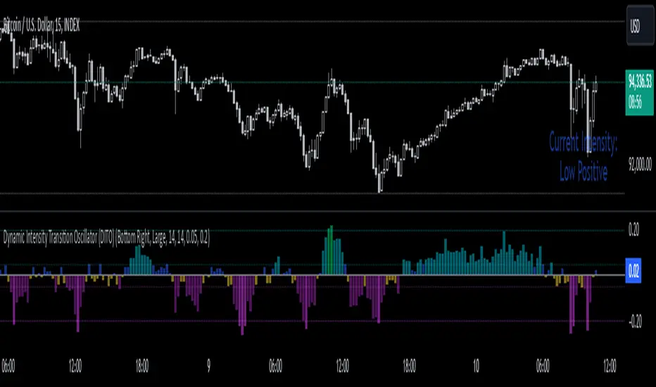
Dynamic Intensity Transition Oscillator (DITO)The Dynamic Intensity Transition Oscillator (DITO) is a comprehensive indicator designed to identify and visualize the slope of price action normalized by volatility, enabling consistent comparisons across different assets. This indicator calculates and categorizes the intensity of price movement into six states—three positive and three negative—while providing visual cues and alerts for state transitions.
Components and Functionality
1. Slope Calculation
- The slope represents the rate of change in price action over a specified period (Slope Calculation Period).
- It is calculated as the difference between the current price and the simple moving average (SMA) of the price, divided by the length of the period.
2. Normalization Using ATR
- To standardize the slope across assets with different price scales and volatilities, the slope is divided by the Average True Range (ATR).
- The ATR ensures that the slope is comparable across assets with varying price levels and volatility.
3. Intensity Levels
- The normalized slope is categorized into six distinct intensity levels:
High Positive: Strong upward momentum.
Medium Positive: Moderate upward momentum.
Low Positive: Weak upward movement or consolidation.
Low Negative: Weak downward movement or consolidation.
Medium Negative: Moderate downward momentum.
High Negative: Strong downward momentum.
4. Visual Representation
- The oscillator is displayed as a histogram, with each intensity level represented by a unique color:
High Positive: Lime green.
Medium Positive: Aqua.
Low Positive: Blue.
Low Negative: Yellow.
Medium Negative: Purple.
High Negative: Fuchsia.
Threshold levels (Low Intensity, Medium Intensity) are plotted as horizontal dotted lines for visual reference, with separate colors for positive and negative thresholds.
5. Intensity Table
- A dynamic table is displayed on the chart to show the current intensity level.
- The table's text color matches the intensity level color for easy interpretation, and its size and position are customizable.
6. Alerts for State Transitions
- The indicator includes a robust alerting system that triggers when the intensity level transitions from one state to another (e.g., from "Medium Positive" to "High Positive").
- The alert includes both the previous and current states for clarity.
Inputs and Customization
The DITO indicator offers a variety of customizable settings:
Indicator Parameters
Slope Calculation Period: Defines the period over which the slope is calculated.
ATR Calculation Period: Defines the period for the ATR used in normalization.
Low Intensity Threshold: Threshold for categorizing weak momentum.
Medium Intensity Threshold: Threshold for categorizing moderate momentum.
Intensity Table Settings
Table Position: Allows you to position the intensity table anywhere on the chart (e.g., "Bottom Right," "Top Left").
Table Size: Enables customization of table text size (e.g., "Small," "Large").
Use Cases
Trend Identification:
- Quickly assess the strength and direction of price movement with color-coded intensity levels.
Cross-Asset Comparisons:
- Use the normalized slope to compare momentum across different assets, regardless of price scale or volatility.
Dynamic Alerts:
- Receive timely alerts when the intensity transitions, helping you act on significant momentum changes.
Consolidation Detection:
- Identify periods of low intensity, signaling potential reversals or breakout opportunities.
How to Use
- Add the indicator to your chart.
- Configure the input parameters to align with your trading strategy.
Observe:
The Oscillator: Use the color-coded histogram to monitor price action intensity.
The Intensity Table: Track the current intensity level dynamically.
Alerts: Respond to state transitions as notified by the alerts.
Final Notes
The Dynamic Intensity Transition Oscillator (DITO) combines trend strength detection, cross-asset comparability, and real-time alerts to offer traders an insightful tool for analyzing market conditions. Its user-friendly visualization and comprehensive alerting make it suitable for both novice and advanced traders.
Disclaimer: This indicator is for educational purposes and is not financial advice. Always perform your own analysis before making trading decisions.
Average Price Range Screener [KFB Quant]Average Price Range Screener
Overview:
The Average Price Range Screener is a technical analysis tool designed to provide insights into the average price volatility across multiple symbols over user-defined time periods. The indicator compares price ranges from different assets and displays them in a visual table and chart for easy reference. This can be especially helpful for traders looking to identify symbols with high or low volatility across various time frames.
Key Features:
Multiple Symbols Supported:
The script allows for analysis of up to 10 symbols, such as major cryptocurrencies and market indices. Symbols can be selected by the user and configured for tracking price volatility.
Dynamic Range Calculation:
The script calculates the average price range of each symbol over three distinct time periods (default are 30, 60, and 90 bars). The price range for each symbol is calculated as a percentage of the bar's high-to-low difference relative to its low value.
Range Visualization:
The results are visually represented using:
- A color-coded table showing the calculated average ranges of each symbol and the current chart symbol.
- A line plot that visually tracks the volatility for each symbol on the chart, with color gradients representing the range intensity from low (red/orange) to high (blue/green).
Customizable Inputs:
- Length Inputs: Users can define the time lengths (default are 30, 60, and 90 bars) for calculating average price ranges for each symbol.
- Symbol Inputs: 10 symbols can be tracked at once, with default values set to popular crypto pairs and indices.
- Color Inputs: Users can customize the color scheme for the range values displayed in the table and chart.
Real-Time Ranking:
The indicator ranks symbols by their average price range, providing a clear view of which assets are exhibiting higher volatility at any given time.
Each symbol's range value is color-coded based on its relative volatility within the selected symbols (using a gradient from low to high range).
Data Table:
The table shows the average range values for each symbol in real-time, allowing users to compare volatility across multiple assets at a glance. The table is dynamically updated as new data comes in.
Interactive Labels:
The indicator adds labels to the chart, showing the average range for each symbol. These labels adjust in real-time as the price range values change, giving users an immediate view of volatility rankings.
How to Use:
Set Time Periods: Adjust the time periods (lengths) to match your trading strategy's timeframe and volatility preference.
Symbol Selection: Add and track the price range for your preferred symbols (cryptocurrencies, stocks, indices).
Monitor Volatility: Use the visual table and plot to identify symbols with higher or lower volatility, and adjust your trading strategy accordingly.
Interpret the Table and Chart: Ranges that are color-coded from red/orange (lower volatility) to blue/green (higher volatility) allow you to quickly gauge which symbols are most volatile.
Disclaimer: This tool is provided for informational and educational purposes only and should not be considered as financial advice. Always conduct your own research and consult with a licensed financial advisor before making any investment decisions.

Market Bias IndicatorOverview
This Pine Script™ code generates a "Market Sentiment Dashboard" on TradingView, providing a visual summary of market sentiment across multiple timeframes. This tool aids traders in making informed decisions by displaying real-time sentiment analysis based on Exponential Moving Averages (EMA).
Key Features
Panel Positioning:
Custom Placement: Traders can position the dashboard at the top, middle, or bottom of the chart and align it to the left, centre, or right, ensuring optimal integration with other chart elements.
Customizable Colours:
Sentiment Colours: Users can define colours for bullish, bearish, and neutral market conditions, enhancing the dashboard's readability.
Text Colour: Customizable text colour ensures clarity against various background colours.
Label Size:
Scalable Labels: Adjustable label sizes (from very small to very large) ensure readability across different screen sizes and resolutions.
Market Sentiment Calculation:
EMA-Based Sentiment: The dashboard calculates sentiment using a 9-period EMA. If the EMA is higher than two bars ago, the sentiment is bullish; if lower, it's bearish; otherwise, it's neutral.
Multiple Timeframes: Sentiment is calculated for several timeframes: 30 minute, 1 hour, 4 hour, 6 hour, 8 hour, 12 hour, 1 day, and 1 week. This broad analysis provides a comprehensive view of market conditions.
Dynamic Table:
Structured Display: The dashboard uses a table to organize and display sentiment data clearly.
Real-Time Updates: The table updates in real-time, providing traders with up-to-date market information.
How It Works
EMA Calculation: The script requests EMA(9) values for each specified timeframe and compares the current EMA with the EMA from two bars ago to determine market sentiment.
Colour Coding: Depending on the sentiment (Bullish, Bearish, or Neutral), the corresponding cell in the table is color-coded using predefined colours.
Table Display: The table displays the timeframe and corresponding sentiment, allowing traders to quickly assess market trends.
Benefits to Traders
Quick Assessment: Traders can quickly evaluate market sentiment across multiple timeframes without switching charts or manually calculating indicators.
Enhanced Visualization: The color-coded sentiment display makes it easy to identify trends at a glance.
Multi-Timeframe Analysis: Provides a broad view of short-term and long-term market trends, helping traders confirm trends and avoid false signals.
This dashboard enhances the overall trading experience by providing a comprehensive, customizable, and easy-to-read summary of market sentiment.
Usage Instructions
Add the Script to Your Chart: Apply the "Market Sentiment Dashboard" indicator to your TradingView chart.
Customize Settings: Adjust the panel position, colours, and label sizes to fit your preferences.
Interpret Sentiment: Use the color-coded table to quickly understand the market sentiment across different timeframes and make informed trading decisions.
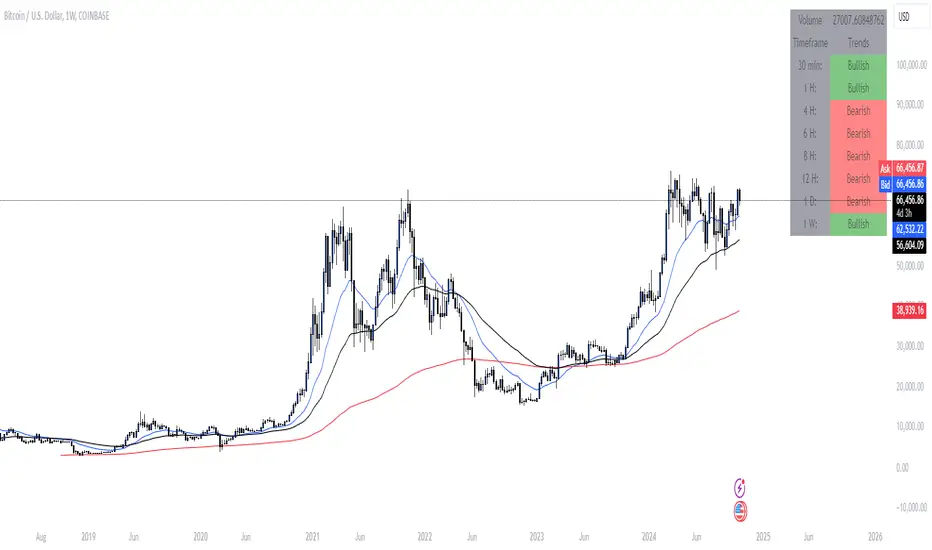
Burst PowerThe Burst Power indicator is to be used for Indian markets where most stocks have a maximum price band limit of 20%.
This indicator is intended to identify stocks with high potential for significant price movements. By analysing historical price action over a user-defined lookback period, it calculates a Burst Power score that reflects the stock's propensity for rapid and substantial moves. This can be helpful for stock selection in strategies involving momentum bursts, swing trading, or identifying stocks with explosive potential.
Key Components
____________________
Significant Move Counts:
5% Moves: Counts the number of days within the lookback period where the stock had a positive close-to-close move between 5% and 10%.
10% Moves: Counts the number of days with a positive close-to-close move between 10% and 19%.
19% Moves: Counts the number of days with a positive close-to-close move of 19% or more.
Maximum Price Move (%):
Identifies the largest positive close-to-close percentage move within the lookback period, along with the date it occurred.
Burst Power Score:
A composite score calculated using the counts of significant moves: Burst Power =(Count5%/5) +(Count10%/2) + (Count19%/0.5)
The score is then rounded to the nearest whole number.
A higher Burst Power score indicates a higher frequency of significant price bursts.
Visual Indicators:
Table Display: Presents all the calculated data in a customisable table on the chart.
Markers on Chart: Plots markers on the chart where significant moves occurred, aiding visual analysis.
Using the Lookback Period
____________________________
The lookback period determines how much historical data the indicator analyses. Users can select from predefined options:
3 Months
6 Months
1 Year
3 Years
5 Years
A shorter lookback period focuses on recent price action, which may be more relevant for short-term trading strategies. A longer lookback period provides a broader historical context, useful for identifying long-term patterns and behaviors.
Interpreting the Burst Power Score
__________________________________
High Burst Power Score (≥15):
Indicates the stock frequently experiences significant price moves.
Suitable for traders seeking quick momentum bursts and swing trading opportunities.
Stocks with high scores may be more volatile but offer potential for rapid gains.
Moderate Burst Power Score (10 to 14):
Suggests occasional significant price movements.
May suit traders looking for a balance between volatility and stability.
Low Burst Power Score (<10):
Reflects fewer significant price bursts.
Stocks are more likely to exhibit longer, sustainable, but slower price trends.
May be preferred by traders focusing on steady growth or longer-term investments.
Note: Trading involves uncertainties, and the Burst Power score should be considered as one of many factors in a comprehensive trading strategy. It is essential to incorporate broader market analysis and risk management practices.
Customisation Options
_________________________
The indicator offers several customisation settings to tailor the display and functionality to individual preferences:
Display Mode:
Full Mode: Shows the detailed table with all components, including significant move counts, maximum price move, and the Burst Power score.
Mini Mode: Displays only the Burst Power score and its corresponding indicator (green, orange, or red circle).
Show Latest Date Column:
Toggle the display of the "Latest Date" column in the table, which shows the most recent occurrence of each significant move category.
Theme (Dark Mode):
Switch between Dark Mode and Light Mode for better visual integration with your chart's color scheme.
Table Position and Size:
Position: Place the table at various locations on the chart (top, middle, bottom; left, center, right).
Size: Adjust the table's text size (tiny, small, normal, large, huge, auto) for optimal readability.
Header Size: Customise the font size of the table headers (Small, Medium, Large).
Color Settings:
Disable Colors in Table: Option to display the table without background colors, which can be useful for printing or if colors are distracting.
Bullish Closing Filter:
Another customisation here is to count a move only when the closing for the day is strong. For this, we have an additional filter to see if close is within the chosen % of the range of the day. Closing within the top 1/3, for instance, indicates a way more bullish day tha, say, closing within the bottom 25%.
Move Markers on chart:
The indicator also marks out days with significant moves. You can choose to hide or show the markers on the candles/bars.
Practical Applications
________________________
Momentum Trading: High Burst Power scores can help identify stocks that are likely to experience rapid price movements, suitable for momentum traders.
Swing Trading: Traders looking for short- to medium-term opportunities may focus on stocks with moderate to high Burst Power scores.
Positional Trading: Lower Burst Power scores may indicate steadier stocks that are less prone to volatility, aligning with long-term investment strategies.
Risk Management: Understanding a stock's propensity for significant moves can aid in setting appropriate stop-loss and take-profit levels.
Disclaimer: Trading involves significant risk, and past performance is not indicative of future results. The Burst Power indicator is intended for educational purposes and should not be construed as financial advice. Always conduct thorough research and consult with a qualified financial professional before making investment decisions.

Interest Rate Trading (Manually Added Rate Decisions) [TANHEF]Interest Rate Trading: How Interest Rates Can Guide Your Next Move.
How were interest rate decisions added?
All interest rate decision dates were manually retrieved from the 'Record of Policy Actions' and 'Minutes of Actions' on the Federal Reserve's website due to inconsistent dates from other sources. These were manually added as Pine Script currently only identifies rate changes, not pauses.
█ Simple Explanation:
This script is designed for analyzing and backtesting trading strategies based on U.S. interest rate decisions which occur during Federal Open Market Committee (FOMC) meetings, to make trading decisions. No trading strategy is perfect, and it's important to understand that expectations won't always play out. The script leverages historical interest rate changes, including increases, decreases, and pauses, across multiple economic time periods from 1971 to the present. The tool integrates two key data sources for interest rates—USINTR and FEDFUNDS—to support decision-making around rate-based trades. The focus is on identifying opportunities and tracking trades driven by interest rate movements.
█ Interest Rate Decision Sources:
As noted above, each decision date has been manually added from the 'Record of Policy Actions' and 'Minutes of Actions' documents on the Federal Reserve's website. This includes +50 years of more than 600 rate decisions.
█ Interest Rate Data Sources:
USINTR: Reflects broader U.S. interest rate trends, including Treasury yields and various benchmarks. This is the preferred option as it corresponds well to the rate decision dates.
FEDFUNDS: Tracks the Federal Funds Rate, which is a more specific rate targeted by the Federal Reserve. This does not change on the exact same days as the rate decisions that occur at FOMC meetings.
█ Trade Criteria:
A variety of trading conditions are predefined to suit different trading strategies. These conditions include:
Increase/Decrease: Standard rate increases or decreases.
Double/Triple Increase/Decrease: A series of consecutive changes.
Aggressive Increase/Decrease: Rate changes that exceed recent movements.
Pause: Identification of no changes (pauses) between rate decisions, including double or triple pauses.
Complex Patterns: Combinations of pauses, increases, or decreases, such as "Pause after Increase" or "Pause or Increase."
█ Trade Execution and Exit:
The script allows automated trade execution based on selected criteria:
Auto-Entry: Option to enter trades automatically at the first valid period.
Max Trade Duration: Optional exit of trades after a specified number of bars (candles).
Pause Days: Minimum duration (in days) to validate rate pauses as entry conditions. This is especially useful for earlier periods (prior to the 2000s), where rate decisions often seemed random compared to the consistency we see today.
█ Visualization:
Several visual elements enhance the backtesting experience:
Time Period Highlighting: Economic time periods are visually segmented on the chart, each with a unique color. These periods include historical phases such as "Stagflation (1971-1982)" and "Post-Pandemic Recovery (2021-Present)".
Trade and Holding Results: Displays the profit and loss of trades and holding results directly on the chart.
Interest Rate Plot: Plots the interest rate movements on the chart, allowing for real-time tracking of rate changes.
Trade Status: Highlights active long or short positions on the chart.
█ Statistics and Criteria Display:
Stats Table: Summarizes trade results, including wins, losses, and draw percentages for both long and short trades.
Criteria Table: Lists the selected entry and exit criteria for both long and short positions.
█ Economic Time Periods:
The script organizes interest rate decisions into well-defined economic periods, allowing traders to backtest strategies specific to historical contexts like:
(1971-1982) Stagflation
(1983-1990) Reaganomics and Deregulation
(1991-1994) Early 1990s (Recession and Recovery)
(1995-2001) Dot-Com Bubble
(2001-2006) Housing Boom
(2007-2009) Global Financial Crisis
(2009-2015) Great Recession Recovery
(2015-2019) Normalization Period
(2019-2021) COVID-19 Pandemic
(2021-Present) Post-Pandemic Recovery
█ User-Configurable Inputs:
Rate Source Selection: Choose between USINTR or FEDFUNDS as the primary interest rate source.
Trade Criteria Customization: Users can select the criteria for long and short trades, specifying when to enter or exit based on changes in the interest rate.
Time Period: Select the time period that you want to isolate testing a strategy with.
Auto-Entry and Pause Settings: Options to automatically enter trades and specify the number of days to confirm a rate pause.
Max Trade Duration: Limits how long trades can remain open, defined by the number of bars.
█ Trade Logic:
The script manages entries and exits for both long and short trades. It calculates the profit or loss percentage based on the entry and exit prices. The script tracks ongoing trades, dynamically updating the profit or loss as price changes.
█ Examples:
One of the most popular opinions is that when rate starts begin you should sell, then buy back in when rate cuts stop dropping. However, this can be easily proven to be a difficult task. Predicting the end of a rate cut is very difficult to do with the the exception that assumes rates will not fall below 0.25%.
2001-2009
Trade Result: +29.85%
Holding Result: -27.74%
1971-2024
Trade Result: +533%
Holding Result: +5901%
█ Backtest and Real-Time Use:
This backtester is useful for historical analysis and real-time trading. By setting up various entry and exit rules tied to interest rate movements, traders can test and refine strategies based on real historical data and rate decision trends.
This powerful tool allows traders to customize strategies, backtest them through different economic periods, and get visual feedback on their trading performance, helping to make more informed decisions based on interest rate dynamics. The main goal of this indicator is to challenge the belief that future events must mirror the 2001 and 2007 rate cuts. If everyone expects something to happen, it usually doesn’t.
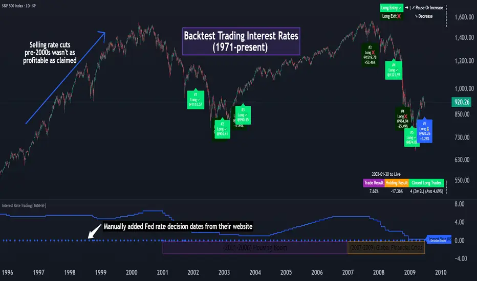
Ticker Tape█ OVERVIEW
This indicator creates a dynamic, scrolling display of multiple securities' latest prices and daily changes, similar to the ticker tapes on financial news channels and the Ticker Tape Widget . It shows realtime market information for a user-specified list of symbols along the bottom of the main chart pane.
█ CONCEPTS
Ticker tape
Traditionally, a ticker tape was a continuous, narrow strip of paper that displayed stock prices, trade volumes, and other financial and security information. Invented by Edward A. Calahan in 1867, ticker tapes were the earliest method for electronically transmitting live stock market data.
A machine known as a "stock ticker" received stock information via telegraph, printing abbreviated company names, transaction prices, and other information in a linear sequence on the paper as new data came in. The term "ticker" in the name comes from the "tick" sound the machine made as it printed stock information. The printed tape provided a running record of trading activity, allowing market participants to stay informed on recent market conditions without needing to be on the exchange floor.
In modern times, electronic displays have replaced physical ticker tapes. However, the term "ticker" remains persistent in today's financial lexicon. Nowadays, ticker symbols and digital tickers appear on financial news networks, trading platforms, and brokerage/exchange websites, offering live updates on market information. Modern electronic displays, thankfully, do not rely on telegraph updates to operate.
█ FEATURES
Requesting a list of securities
The "Symbol list" text box in the indicator's "Settings/Inputs" tab allows users to list up to 40 symbols or ticker Identifiers. The indicator dynamically requests and displays information for each one. To add symbols to the list, enter their names separated by commas . For example: "BITSTAMP:BTCUSD, TSLA, MSFT".
Each item in the comma-separated list must represent a valid symbol or ticker ID. If the list includes an invalid symbol, the script will raise a runtime error.
To specify a broker/exchange for a symbol, include its name as a prefix with a colon in the "EXCHANGE:SYMBOL" format. If a symbol in the list does not specify an exchange prefix, the indicator selects the most commonly used exchange when requesting the data.
Realtime updates
This indicator requests symbol descriptions, current market prices, daily price changes, and daily change percentages for each ticker from the user-specified list of symbols or ticker identifiers. It receives updated information for each security after new realtime ticks on the current chart.
After a new realtime price update, the indicator updates the values shown in the tape display and their colors.
The color of the percentages in the tape depends on the change in price from the previous day . The text is green when the daily change is positive, red when the value is negative, and gray when the value is 0.
The color of each displayed price depends on the change in value from the last recorded update, not the change over a daily period. For example, if a security's price increases in the latest update, the ticker tape shows that price with green text, even if the current price is below the previous day's closing price. This behavior allows users to monitor realtime directional changes in the requested securities.
NOTE: Pine scripts execute on realtime bars when new ticks are available in the chart's data feed. If no new updates are available from the chart's realtime feed, it may cause a delay in the data the indicator receives.
Ticker motion
This indicator's tape display shows a list of security information that incrementally scrolls horizontally from right to left after new chart updates, providing a dynamic visual stream of current market data. The scrolling effect works by using a counter that increments across successive intervals after realtime ticks to control the offset of each listed security. Users can set the initial scroll offset with the "Offset" input in the "Settings/Inputs" tab.
The scrolling rate of the ticker tape display depends on the realtime ticks available from the chart's data feed. Using the indicator on a chart with frequent realtime updates results in smoother scrolling. If no new realtime ticks are available in the chart's feed, the ticker tape does not move. Users can also deactivate the scrolling feature by toggling the "Running" input in the indicator's settings.
█ FOR Pine Script™ CODERS
• This script utilizes dynamic requests to iteratively fetch information from multiple contexts using a single request.security() instance in the code. Previously, `request.*()` functions were not allowed within the local scopes of loops or conditional structures, and most `request.*()` function parameters, excluding `expression`, required arguments of a simple or weaker qualified type. The new `dynamic_requests` parameter in script declaration statements enables more flexibility in how scripts can use `request.*()` calls. When its value is `true`, all `request.*()` functions can accept series arguments for the parameters that define their requested contexts, and `request.*()` functions can execute within local scopes. See the Dynamic requests section of the Pine Script™ User Manual to learn more.
• Scripts can execute up to 40 unique `request.*()` function calls. A `request.*()` call is unique only if the script does not already call the same function with the same arguments. See this section of the User Manual's Limitations page for more information.
• This script converts a comma-separated "string" list of symbols or ticker IDs into an array . It then loops through this array, dynamically requesting data from each symbol's context and storing the results within a collection of custom `Tape` objects . Each `Tape` instance holds information about a symbol, which the script uses to populate the table that displays the ticker tape.
• This script uses the varip keyword to declare variables and `Tape` fields that update across ticks on unconfirmed bars without rolling back. This behavior allows the script to color the tape's text based on the latest price movements and change the locations of the table cells after realtime updates without reverting. See the `varip` section of the User Manual to learn more about using this keyword.
• Typically, when requesting higher-timeframe data with request.security() using barmerge.lookahead_on as the `lookahead` argument, the `expression` argument should use the history-referencing operator to offset the series, preventing lookahead bias on historical bars. However, the request.security() call in this script uses barmerge.lookahead_on without offsetting the `expression` because the script only displays results for the latest historical bar and all realtime bars, where there is no future information to leak into the past. Instead, using this call on those bars ensures each request fetches the most recent data available from each context.
• The request.security() instance in this script includes a `calc_bars_count` argument to specify that each request retrieves only a minimal number of bars from the end of each symbol's historical data feed. The script does not need to request all the historical data for each symbol because it only shows results on the last chart bar that do not depend on the entire time series. In this case, reducing the retrieved bars in each request helps minimize resource usage without impacting the calculated results.
Look first. Then leap.
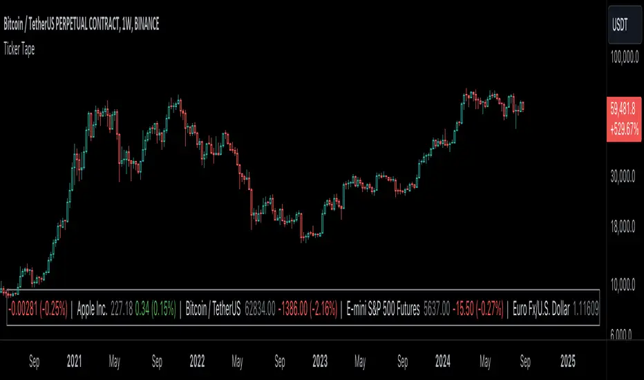
Uptrick: TimeFrame Trends: Performance & Sentiment Indicator### **Uptrick: TimeFrame Trends: Performance & Sentiment Indicator (TFT) - In-Depth Explanation**
#### **Overview**
The **Uptrick: TimeFrame Trends: Performance & Sentiment Indicator (TFT)** is a sophisticated trading tool designed to provide traders with a comprehensive view of market trends across multiple timeframes, combined with a sentiment gauge through the Relative Strength Index (RSI). This indicator offers a unique blend of performance analysis, sentiment evaluation, and visual signal generation, making it an invaluable resource for traders who seek to understand both the macro and micro trends within a financial instrument.
#### **Purpose**
The primary purpose of the TFT indicator is to empower traders with the ability to assess the performance of an asset over various timeframes while simultaneously gauging market sentiment through the RSI. By analyzing price changes over periods ranging from one week to one year, and complementing this with sentiment signals, TFT enables traders to make informed decisions based on a well-rounded analysis of historical price performance and current market conditions.
#### **Key Components and Features**
1. **Multi-Timeframe Performance Analysis:**
- **Performance Lookback Periods:**
- The TFT indicator calculates the percentage price change over several predefined timeframes: 7 days (1 week), 14 days (2 weeks), 30 days (1 month), 180 days (6 months), and 365 days (1 year). These timeframes provide a layered view of how an asset has performed over short, medium, and long-term periods.
- **Percentage Change Calculation:**
- The indicator computes the percentage change for each timeframe by comparing the current closing price to the closing price at the start of each period. This gives traders insight into the strength and direction of the trend over different periods, helping them identify consistent trends or potential reversals.
2. **Sentiment Analysis Using RSI:**
- **Relative Strength Index (RSI):**
- RSI is a widely-used momentum oscillator that measures the speed and change of price movements. It oscillates between 0 and 100 and is typically used to identify overbought or oversold conditions. In TFT, the RSI is calculated using a 14-period lookback, which is standard for most RSI implementations.
- **RSI Smoothing with EMA:**
- To refine the RSI signal and reduce noise, TFT applies a 10-period Exponential Moving Average (EMA) to the RSI values. This smoothed RSI is then used to generate buy, sell, and neutral signals based on its position relative to the 50 level:
- **Buy Signal:** Triggered when the smoothed RSI crosses above 50, indicating bullish sentiment.
- **Sell Signal:** Triggered when the smoothed RSI crosses below 50, indicating bearish sentiment.
- **Neutral Signal:** Triggered when the smoothed RSI equals 50, suggesting indecision or a balanced market.
3. **Visual Signal Generation:**
- **Signal Plots:**
- TFT provides clear visual cues directly on the price chart by plotting shapes at the points where buy, sell, or neutral signals are generated. These shapes are color-coded (green for buy, red for sell, yellow for neutral) and are positioned below or above the price bars for easy identification.
- **First Occurrence Trigger:**
- To avoid clutter and focus on significant market shifts, TFT only triggers the first occurrence of each signal type. This feature helps traders concentrate on the most relevant signals without being overwhelmed by repeated alerts.
4. **Customizable Performance & Sentiment Table:**
- **Table Display:**
- The TFT indicator includes a customizable table that displays the calculated percentage changes for each timeframe. This table is positioned on the chart according to user preference (top-left, top-right, bottom-left, bottom-right) and provides a quick reference to the asset’s performance across multiple periods.
- **Dynamic Text Color:**
- To enhance readability and provide immediate visual feedback, the text color in the table changes based on the direction of the percentage change: green for positive (upward movement) and red for negative (downward movement). This color-coding helps traders quickly assess whether the asset is in an uptrend or downtrend for each period.
- **Customizable Font Size:**
- Traders can adjust the font size of the table to fit their chart layout and personal preferences, ensuring that the information is accessible without being intrusive.
5. **Flexibility and Customization:**
- **Lookback Period Customization:**
- While the default lookback periods are set for common trading intervals (7 days, 14 days, etc.), these can be adjusted to match different trading strategies or market conditions. This flexibility allows traders to tailor the indicator to focus on the timeframes most relevant to their analysis.
- **RSI and EMA Settings:**
- The length of the RSI calculation and the smoothing EMA can also be customized. This is particularly useful for traders who prefer shorter or longer periods for their momentum analysis, allowing them to fine-tune the sensitivity of the indicator.
- **Table Position and Appearance:**
- The table’s position on the chart, along with its font size and colors, is fully customizable. This ensures that the indicator can be integrated seamlessly into any chart setup without obstructing key price data.
#### **Use Cases and Applications**
1. **Trend Identification and Confirmation:**
- **Short-Term Traders:**
- Traders focused on short-term movements can use the 7-day and 14-day performance metrics to identify recent trends and momentum shifts. The RSI signals provide additional confirmation, helping traders enter or exit positions based on the latest market sentiment.
- **Swing Traders:**
- For those holding positions over days to weeks, the 30-day and 180-day performance data are particularly useful. These metrics highlight medium-term trends, and when combined with RSI signals, they provide a robust framework for swing trading strategies.
- **Long-Term Investors:**
- Long-term investors can benefit from the 1-year performance data to gauge the overall health and direction of an asset. The indicator’s ability to track performance across different periods helps in identifying long-term trends and potential reversal points.
2. **Sentiment Analysis and Market Timing:**
- **Market Sentiment Tracking:**
- By using RSI in conjunction with performance metrics, TFT provides a clear picture of market sentiment. Traders can use this information to time their entries and exits more effectively, aligning their trades with periods of strong bullish or bearish sentiment.
- **Avoiding False Signals:**
- The smoothing of RSI helps reduce noise and avoid false signals that are common in volatile markets. This makes the TFT indicator a reliable tool for identifying true market trends and avoiding whipsaws that can lead to losses.
3. **Comprehensive Market Analysis:**
- **Multi-Timeframe Analysis:**
- TFT’s ability to analyze multiple timeframes simultaneously makes it an excellent tool for comprehensive market analysis. Traders can compare short-term and long-term performance to understand the broader market context, making it easier to align their trading strategies with the overall trend.
- **Performance Benchmarking:**
- The percentage change metrics provide a clear benchmark for an asset’s performance over time. This information can be used to compare the asset against broader market indices or other assets, helping traders make more informed decisions about where to allocate their capital.
4. **Custom Strategy Development:**
- **Tailoring to Specific Markets:**
- TFT can be customized to suit different markets, whether it’s stocks, forex, commodities, or cryptocurrencies. For instance, traders in volatile markets may opt for shorter lookback periods and more sensitive RSI settings, while those in stable markets may prefer longer periods for a smoother analysis.
- **Integrating with Other Indicators:**
- TFT can be used alongside other technical indicators to create a more comprehensive trading strategy. For example, combining TFT with moving averages, Bollinger Bands, or MACD can provide additional layers of confirmation and reduce the likelihood of false signals.
#### **Best Practices for Using TFT**
- **Regularly Adjust Lookback Periods:**
- Depending on the market conditions and the asset being traded, it’s important to regularly review and adjust the lookback periods for the performance metrics. This ensures that the indicator remains relevant and responsive to current market trends.
- **Combine with Volume Analysis:**
- While TFT provides a solid foundation for trend and sentiment analysis, combining it with volume indicators can further enhance its effectiveness. Volume can confirm the strength of a trend or signal potential reversals when divergences occur.
- **Use RSI with Other Momentum Indicators:**
- Although RSI is a powerful tool on its own, using it alongside other momentum indicators like Stochastic Oscillator or MACD can provide additional confirmation and help refine entry and exit points.
- **Customize Table Settings for Clarity:**
- Ensure that the performance table is positioned and sized appropriately on the chart. It should be easily readable without obstructing important price data. Adjust the text size and colors as needed to maintain clarity.
- **Monitor Multiple Timeframes:**
- Utilize the multi-timeframe analysis feature of TFT to monitor trends across different periods. This helps in identifying the dominant trend and avoiding trades that go against the broader market direction.
#### **Conclusion**
The **Uptrick: TimeFrame Trends: Performance & Sentiment Indicator (TFT)** is a comprehensive and versatile tool that combines the power of multi-timeframe performance analysis with sentiment gauging through RSI. Its ability to customize and adapt to various trading strategies and markets makes it a valuable asset for traders at all levels. By offering a clear visual representation of trends and market sentiment, TFT empowers traders to make more informed and confident trading decisions, whether they are focusing on short-term price movements or long-term investment opportunities. With its deep integration of performance metrics and sentiment analysis, TFT stands out as a must-have indicator for any trader looking to gain a holistic understanding of market dynamics.
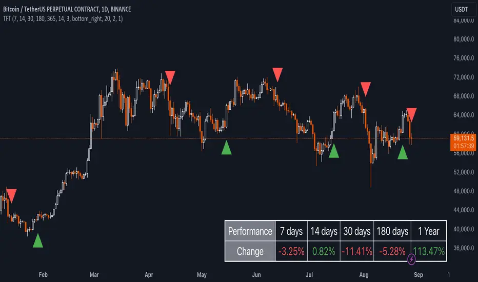
Bearish vs Bullish ArgumentsThe Bearish vs Bullish Arguments Indicator is a tool designed to help traders visually assess and compare the number of bullish and bearish arguments based on their custom inputs. This script enables users to input up to five bullish and five bearish arguments, dynamically displaying the bias on a clean and customizable table on the chart. This provides traders with a clear, visual representation of the market sentiment they have identified.
Key Features:
Customizable Inputs: Users can input up to five bullish and five bearish arguments, which are displayed in a table on the chart.
Bias Calculation: The script calculates the bias (Bullish, Bearish, or Neutral) based on the number of bullish and bearish arguments provided.
Color Customization: Users can customize the colors for the table background, text, and headers, ensuring the table fits seamlessly into their charting environment.
Reset Functionality: A reset switch allows users to clear all input arguments with a single click, making it easy to start fresh.
How It Works:
Input Fields: The script provides input fields for up to five bullish and five bearish arguments. Each input is a simple text field where users can describe their arguments.
Bias Calculation: The script counts the number of non-empty bullish and bearish arguments and determines the overall bias. The bias is displayed in the table with a dynamically changing color to indicate whether the market sentiment is bullish, bearish, or neutral.
Customizable Table: The table is positioned on the chart according to the user's preference (top-left, top-right, bottom-left, bottom-right) and can be customized in terms of background color and text color.
How to Use:
Add the Indicator: Add the Bearish vs Bullish Arguments Indicator to your chart.
Input Arguments: Enter up to five bullish and five bearish arguments in the provided input fields in the script settings.
Customize Appearance: Adjust the table's background color, text color, and position on the chart to fit your preferences.
Example Use Case:
A trader might use this indicator to visually balance their arguments for and against a particular trade setup. By entering their reasons for a bullish outlook in the bullish argument fields and their reasons for a bearish outlook in the bearish argument fields, they can quickly see which side has more supporting points and make a more informed trading decision.
This script was inspired by Arjoio's concepts

Multi-Frame Market Sentiment DashboardOverview
This Pine Script™ code generates a "Market Sentiment Dashboard" on TradingView, providing a visual summary of market sentiment across multiple timeframes. This tool aids traders in making informed decisions by displaying real-time sentiment analysis based on Exponential Moving Averages (EMA).
Key Features
Panel Positioning:
Custom Placement: Traders can position the dashboard at the top, middle, or bottom of the chart and align it to the left, center, or right, ensuring optimal integration with other chart elements.
Customizable Colors:
Sentiment Colors: Users can define colors for bullish, bearish, and neutral market conditions, enhancing the dashboard's readability.
Text Color: Customizable text color ensures clarity against various background colors.
Label Size:
Scalable Labels: Adjustable label sizes (from very small to very large) ensure readability across different screen sizes and resolutions.
Market Sentiment Calculation:
EMA-Based Sentiment: The dashboard calculates sentiment using a 9-period EMA. If the EMA is higher than two bars ago, the sentiment is bullish; if lower, it's bearish; otherwise, it's neutral.
Multiple Timeframes: Sentiment is calculated for several timeframes: 1 minute, 3 minutes, 5 minutes, 15 minutes, 30 minutes, 1 hour, 4 hours, and 1 day. This broad analysis provides a comprehensive view of market conditions.
Dynamic Table:
Structured Display: The dashboard uses a table to organize and display sentiment data clearly.
Real-Time Updates: The table updates in real-time, providing traders with up-to-date market information.
How It Works
EMA Calculation: The script requests EMA(9) values for each specified timeframe and compares the current EMA with the EMA from two bars ago to determine market sentiment.
Color Coding: Depending on the sentiment (Bullish, Bearish, or Neutral), the corresponding cell in the table is color-coded using predefined colors.
Table Display: The table displays the timeframe and corresponding sentiment, allowing traders to quickly assess market trends.
Benefits to Traders
Quick Assessment: Traders can quickly evaluate market sentiment across multiple timeframes without switching charts or manually calculating indicators.
Enhanced Visualization: The color-coded sentiment display makes it easy to identify trends at a glance.
Multi-Timeframe Analysis: Provides a broad view of short-term and long-term market trends, helping traders confirm trends and avoid false signals.
This dashboard enhances the overall trading experience by providing a comprehensive, customizable, and easy-to-read summary of market sentiment.
Usage Instructions
Add the Script to Your Chart: Apply the "Market Sentiment Dashboard" indicator to your TradingView chart.
Customize Settings: Adjust the panel position, colors, and label sizes to fit your preferences.
Interpret Sentiment: Use the color-coded table to quickly understand the market sentiment across different timeframes and make informed trading decisions.
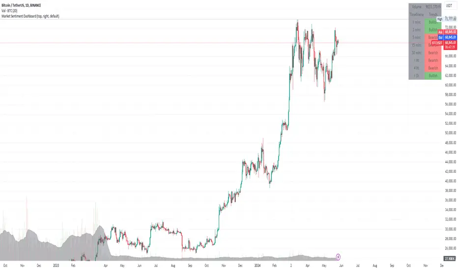
Nadaraya-Watson Probability [Yosiet]The script calculates and displays probability bands around price movements, offering insights into potential market trends.
Setting Up the Script
Window Size: Determines the length of the window for the Nadaraya-Watson estimation. A larger window smooths the data more but might lag current market conditions.
Bandwidth: Controls the bandwidth for the kernel regression, affecting the smoothness of the probability bands.
Reading the Data Table
The script dynamically updates a table positioned at the bottom right of your chart, providing real-time insights into market probabilities. Here's how to interpret the table:
Table Columns: The table is organized into three columns:
Up: Indicates the probability or relative change percentage for the upper band.
Down: Indicates the probability or relative change percentage for the lower band.
Table Rows: There are two main rows of interest:
P%: Shows the price change percentage difference between the bands and the closing price. A positive value in the "Up" column suggests the upper band is above the current close, indicating potential upward momentum. Conversely, a negative value in the "Down" column suggests downward momentum.
R%: Displays the relative inner change percentage difference between the bands, offering a measure of the market's volatility or stability within the bands.
Utilizing the Insights
Market Trends: A widening gap between the "Up" and "Down" percentages in the "P%" row might indicate increasing market volatility. Traders can use this information to adjust their risk management strategies accordingly.
Entry and Exit Points: The "R%" row provides insights into the relative position of the current price within the probability bands. Traders might consider positions closer to the lower band as potential entry points and positions near the upper band as exit points or take-profit levels.
Conclusion
The Nadaraya-Watson Probability script offers a sophisticated tool for traders looking to incorporate statistical analysis into their trading strategy. By understanding and utilizing the data presented in the script's table, traders can gain insights into market trends and volatility, aiding in decision-making processes. Remember, no indicator is foolproof; always consider multiple data sources and analyses when making trading decisions.

Ohlson O-Score IndicatorThe Ohlson O-Score is a financial metric developed by Olof Ohlson to predict the probability of a company experiencing financial distress. It is widely used by investors and analysts as a key tool for financial analysis.
Inputs:
Period: Select the financial period for analysis, either "FY" (Fiscal Year) or "FQ" (Fiscal Quarter).
Country: Specify the country for Gross Net Product data. This helps in tailoring the analysis to specific economic conditions.
Gross Net Product : Define the number of years back for the index to be set at 100. This parameter provides a historical context for the analysis.
Table Display : Customize the display of various tables to suit your preference and analytical needs.
Key Features:
Predictive Power : The Ohlson O-Score is renowned for its predictive power in assessing the financial health of a company. It incorporates multiple financial ratios and indicators to provide a comprehensive view.
Financial Distress Prediction : Use the O-Score to gauge the likelihood of a company facing financial distress in the future. It's a valuable tool for risk assessment.
Country-Specific Analysis : Tailor the analysis to the economic conditions of a specific country, ensuring a more accurate evaluation of financial health.
Historical Context : Set the Gross Net Product index at a specific historical point, allowing for a deeper understanding of how a company's financial health has evolved over time.
How to Use:
Select Period : Choose either Fiscal Year or Fiscal Quarter based on your preference.
Specify Country : Input the country for country-specific Gross Net Product data.
Set Historical Context : Determine the number of years back for the index to be set at 100, providing historical context to your analysis.
Custom Table Display : Personalize the display of various tables to focus on the metrics that matter most to you.
Calculation and component description
Here is the description of O-score components as found in orginal Ohlson publication :
1. SIZE = log(total assets/GNP price-level index). The index assumes a base value of 100 for 1968. Total assets are as reported in dollars. The index year is as of the year prior to the year of the balance sheet date. The procedure assures a real-time implementation of the model. The log transform has an important implication. Suppose two firms, A and B, have a balance sheet date in the same year, then the sign of PA - Pe is independent of the price-level index. (This will not follow unless the log transform is applied.) The latter is, of course, a desirable property.
2. TLTA = Total liabilities divided by total assets.
3. WCTA = Working capital divided by total assets.
4. CLCA = Current liabilities divided by current assets.
5. OENEG = One if total liabilities exceeds total assets, zero otherwise.
6. NITA = Net income divided by total assets.
7. FUTL = Funds provided by operations divided by total liabilities
8. INTWO = One if net income was negative for the last two years, zero otherwise.
9. CHIN = (NI, - NI,-1)/(| NIL + (NI-|), where NI, is net income for the most recent period. The denominator acts as a level indicator. The variable is thus intended to measure change in net income. (The measure appears to be due to McKibben ).
Interpretation
The foundational model for the O-Score evolved from an extensive study encompassing over 2000 companies, a notable leap from its predecessor, the Altman Z-Score, which examined a mere 66 companies. In direct comparison, the O-Score demonstrates significantly heightened accuracy in predicting bankruptcy within a 2-year horizon.
While the original Z-Score boasted an estimated accuracy of over 70%, later iterations reached impressive levels of 90%. Remarkably, the O-Score surpasses even these high benchmarks in accuracy.
It's essential to acknowledge that no mathematical model achieves 100% accuracy. While the O-Score excels in forecasting bankruptcy or solvency, its precision can be influenced by factors both internal and external to the formula.
For the O-Score, any results exceeding 0.5 indicate a heightened likelihood of the firm defaulting within two years. The O-Score stands as a robust tool in financial analysis, offering nuanced insights into a company's financial stability with a remarkable degree of accuracy.
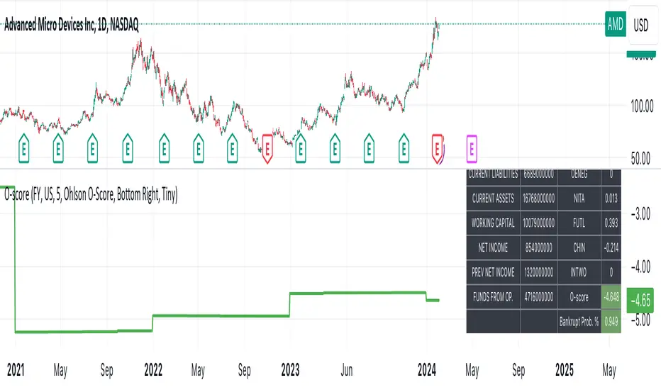
dashboard MTF,EMA User Guide: Dashboard MTF EMA
Script Installation:
Copy the script code.
Go to the script window (Pine Editor) on TradingView.
Paste the code into the script window.
Save the script.
Adding the Script to the Chart:
Return to your chart on TradingView.
Look for the script in the list of available scripts.
Add the script to the chart.
Interpreting the Table:
On the right side of the chart, you will see a table labeled "EMA" with arrows.
The rows correspond to different timeframes: 5 minutes (5M), 15 minutes (15M), 1 hour (1H), 4 hours (4H), and 1 day (1D).
Understanding the Arrows:
Each row of the table has two columns: "EMA" and an arrow.
"EMA" indicates the trend of the Exponential Moving Average (EMA) for the specified period.
The arrow indicates the direction of the trend: ▲ for bullish, ▼ for bearish.
Table Colors:
The colors of the table reflect the current trend based on the comparison between fast and slow EMAs.
Blue (▲) indicates a bullish trend.
Red (▼) indicates a bearish trend.
Table Theme:
The table has a dark (Dark) or light (Light) theme according to your preference.
The background, frame, and colors are adjusted based on the selected theme.
Usage:
Use the table as a quick indicator of trends on different timeframes.
The arrows help you quickly identify trends without navigating between different time units.
Designed to simplify analysis and avoid cluttering the chart with multiple indicators.